Minimizing and Maximizing Maxima and Minima

qbpp::max(f, g) and qbpp::min(f, g) (Nonlinear Functions and Native Constraints) represent the maximum and the minimum of two expressions. Since the solvers minimize the energy, adding them to the objective with a positive coefficient works toward minimizing, and with a negative coefficient toward maximizing, which gives four uses:

Term added to the objective	Meaning
`qbpp::max(f, g)`	minimize the maximum
`-qbpp::max(f, g)`	maximize the maximum
`qbpp::min(f, g)`	minimize the minimum
`-qbpp::min(f, g)`	maximize the minimum

This page first explains these four uses for two expressions with graphs, and then explains how to handle the maximum or minimum of three or more expressions.

Two expressions

Consider an integer variable $x$ that takes values from 0 to 63 and the following two functions:

\[f(x) = (x - 33)^2 + 1000, \qquad g(x) = 2109 - (x - 30)^2\]

$f$ is a parabola opening upward and $g$ a parabola opening downward; they cross at $x = 8$ and $x = 55$. In the following figure, the wide gray line shows $\max(f, g)$ on the left and $\min(f, g)$ on the right:

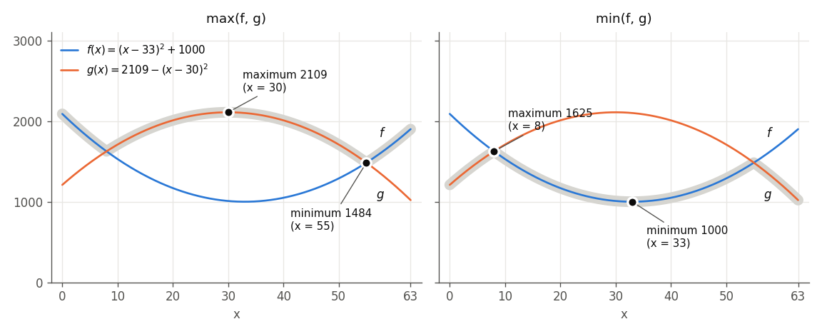
Graphs of f and g; the gray line shows max(f, g) on the left and min(f, g) on the right, with the four answers marked

The four answers are the lowest and highest points of the gray lines:

minimizing qbpp::max(f, g): the lowest point of the left line, the crossing at $x = 55$, 1484
minimizing -qbpp::max(f, g) (maximizing the maximum): the highest point of the left line, the vertex of $g$ at $x = 30$, 2109
minimizing qbpp::min(f, g): the lowest point of the right line, the vertex of $f$ at $x = 33$, 1000
minimizing -qbpp::min(f, g) (maximizing the minimum): the highest point of the right line, the other crossing at $x = 8$, 1625

The following program solves these four cases in turn:

#include <qbpp/exhaustive_solver.hpp>
#include <qbpp/qbpp.hpp>

int main() {
  auto x = 0 <= qbpp::int_var("x") <= 63;
  auto f = qbpp::sqr(x - 33) + 1000;
  auto g = 2109 - qbpp::sqr(x - 30);
  auto solve = [&](const char* name, qbpp::Expr obj) {
    obj.simplify();
    auto sol = qbpp::ExhaustiveSolver(obj).search();
    std::cout << name << ": energy = " << sol.energy() << ", x = " << sol(x)
              << ", f = " << sol(f) << ", g = " << sol(g) << std::endl;
  };
  solve("+max", qbpp::max(f, g));
  solve("-max", -qbpp::max(f, g));
  solve("+min", qbpp::min(f, g));
  solve("-min", -qbpp::min(f, g));
}

solve simplifies the objective obj, finds its exact minimum with ExhaustiveSolver, and prints it.
-qbpp::max(f, g) and -qbpp::min(f, g) are the terms multiplied by the negative coefficient $-1$.

The output of the program is as follows:

+max: energy = 1484, x = 55, f = 1484, g = 1484
-max: energy = -2109, x = 30, f = 1009, g = 2109
+min: energy = 1000, x = 33, f = 1000, g = 2100
-min: energy = -1625, x = 8, f = 1625, g = 1625

For the terms with a negative coefficient, the energy is the maximum (minimum) with the sign reversed.

With two expressions, all four cases are written directly with qbpp::max and qbpp::min, without auxiliary variables. The bundled solvers handle all four correctly. MIP solvers, however, accept only two of them: minimizing the maximum and maximizing the minimum (Nonlinear Functions and Native Constraints).

Three or more expressions

qbpp::max and qbpp::min accept only two expressions; passing three or more (or an array of expressions) is rejected at compile time. Nonlinear functions cannot be nested either, so nesting them as in qbpp::max(qbpp::max(f, g), h) throws an exception.

The maximum or minimum of three or more expressions $f_1, \ldots, f_n$ is expressed by adding auxiliary variables. Which variables to add depends on the case:

	Minimize	Maximize
Maximum $\max(f_1, \ldots, f_n)$	an integer variable $z$ with relu (or cons)	select one with a one-hot
Minimum $\min(f_1, \ldots, f_n)$	select one with a one-hot	an integer variable $z$ with relu (or cons)

The maximum is at most $t$ exactly when every $f_i$ is at most $t$. So to make the maximum small, we use an integer variable $z$ that bounds every $f_i$ from above. On the other hand, the maximum is at least $t$ exactly when at least one $f_i$ is at least $t$. So to make the maximum large, we choose which $f_i$ to use with a one-hot. The minimum is the other way around. Each method works only for its two cases in the table.

This section uses the following three functions, different from those of the previous section ($x$ is again an integer variable from 0 to 63):

\[f(x) = (x - 52)^2 + 300, \qquad g(x) = (x - 14)^2, \qquad h(x) = 3400 - (x - 49)^2\]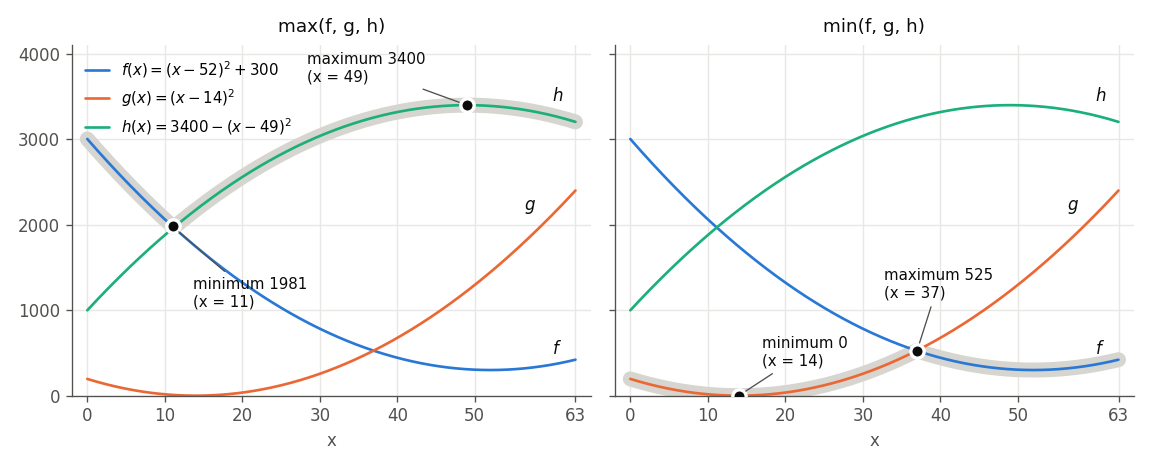

Graphs of f, g, and h; the gray line shows max(f, g, h) on the left and min(f, g, h) on the right, with the four answers marked

Minimizing the maximum and maximizing the minimum

To minimize $\max(f_1, \ldots, f_n)$, minimize the following expression instead:

\[z + 2\sum_{i=1}^{n} \operatorname{relu}(f_i - z)\]

$\operatorname{relu}(f_i - z)$ is the amount by which $f_i$ exceeds $z$. If $z$ is at least the maximum, all relu terms are 0 and the value of the expression is $z$. Lowering $z$ by 1 below the maximum decreases the $z$ part by 1, but the largest expression then exceeds $z$, so the relu terms increase by at least 2. Therefore, this expression is minimized when $z$ is exactly the maximum, and its minimum value equals the maximum.

With weight 1, the minimum value of the expression still equals the maximum, but it is attained for any $z$ between the second largest value and the maximum, so the value of $z$ does not tell the maximum. With a weight larger than 1, $z$ becomes exactly the maximum.

To maximize $\min(f_1, \ldots, f_n)$, minimize the following expression in the same way:

\[-z + 2\sum_{i=1}^{n} \operatorname{relu}(z - f_i)\]

$z$ bounds the minimum from below. The expression is minimized when $z$ is exactly the minimum, and its value is then the minimum with the sign reversed.

The following program solves these two cases for the three functions:

#include <qbpp/exhaustive_solver.hpp>
#include <qbpp/qbpp.hpp>

int main() {
  auto x = 0 <= qbpp::int_var("x") <= 63;
  auto f = qbpp::sqr(x - 52) + 300;
  auto g = qbpp::sqr(x - 14);
  auto h = 3400 - qbpp::sqr(x - 49);
  auto z = 0 <= qbpp::int_var("z") <= 4000;
  auto solve = [&](const char* name, qbpp::Expr obj) {
    obj.simplify();
    auto sol = qbpp::ExhaustiveSolver(obj).search();
    std::cout << name << ": energy = " << sol.energy() << ", z = " << sol(z)
              << ", x = " << sol(x) << ", f = " << sol(f) << ", g = " << sol(g)
              << ", h = " << sol(h) << std::endl;
  };
  solve("+max", z + 2 * qbpp::relu(f - z) + 2 * qbpp::relu(g - z) + 2 * qbpp::relu(h - z));
  solve("-min", -z + 2 * qbpp::relu(z - f) + 2 * qbpp::relu(z - g) + 2 * qbpp::relu(z - h));
}

The values of $f$, $g$, and $h$ are at most 4000, so the range of $z$ is 0 to 4000.

The output of the program is as follows:

+max: energy = 1981, z = 1981, x = 11, f = 1981, g = 9, h = 1956
-min: energy = -525, z = 525, x = 37, f = 525, g = 529, h = 3256

The minimum of the maximum is 1981, the lowest point of the gray line on the left of the figure, at $x = 11$ near where $f$ and $h$ cross; since $x$ is an integer, the minimum is at an integer near the crossing rather than at the crossing itself. The maximum of the minimum is 525, the highest point of the gray line on the right, at $x = 37$ near where $f$ and $g$ cross. In both cases, $z$ takes that value.

Writing it with cons

Alternatively, you can write “every $f_i$ is at most $z$” as constraints and minimize $z$:

\[z + 2\sum_{i=1}^{n} \operatorname{cons}(f_i - z \le 0)\]

In the program above, just replace the relu terms of the "+max" line with 2 * qbpp::cons(f - z <= 0) and so on to get the same result (energy 1981, $z = 1981$). To maximize the minimum, replace the relu terms of the "-min" line with 2 * qbpp::cons(f - z >= 0) and so on.

The value of qbpp::cons() is the square of the violation, so lowering $z$ by $d$ below the maximum increases it by at least $2d^2$. This is more than the decrease $d$ of the $z$ part, so this expression is also minimized when $z$ is exactly the maximum, and its minimum value equals the maximum.

Minimizing the makespan (the time at which the last machine finishes) in Machine Scheduling with Due Dates is an example of this form. The coefficient of $z$ is 100, and the constraint of each machine is written with qbpp::cons() with weight 100000.

Differences between relu and cons

With either method, the minimum is attained when $z$ is exactly the maximum, and the energy there equals the maximum. They differ in two points.

How violations are counted: The part written with qbpp::cons() is treated as constraints. For a solution where $z$ is smaller than the maximum, f.cons(sol), f.violations(sol), and f.is_feasible(sol) count it as a violation, and a search with target_energy does not stop until all constraints are satisfied. The part written with qbpp::relu() is part of the objective and is not counted as constraints. $f_i \le z$ is a condition for expressing the maximum, not a requirement that must be met, so when you only use the maximum in the objective, qbpp::relu() matches the meaning better. qbpp::cons() reads “at most $z$” as a constraint, which is a common way of writing it in mathematical programming.

Shape of the value and the weight: The value of qbpp::cons(f_i - z <= 0) is the same as qbpp::relu(f_i - z, 2), the square of the excess. qbpp::relu(f_i - z) is the excess itself (linear). In both cases, the property above holds if the weight is larger than the coefficient of $z$. The difference shows up in intermediate states of the search where $z$ is slightly smaller than the maximum. When one expression attains the maximum, lowering $z$ by $d$ below the maximum increases the energy by $(\lambda - 1)d$ with relu and by $\lambda d^2 - d$ with cons, where $\lambda$ is the weight. If this increase is small, the solver can try lowering $z$ slightly below the maximum, and every expression exceeding $z$ gets a direction in which “making it smaller lowers the energy”. With a large weight, this state becomes expensive, and the solver mostly moves in the region where $z$ is at least every expression. There the energy depends only on $z$ (that is, on the maximum), so if two or more expressions attain the maximum, making one of them smaller does not change the energy, and the search can become slow for some problems. A weight larger than the coefficient of $z$ is enough (this page uses twice the coefficient).

Maximizing the maximum and minimizing the minimum

To maximize $\max(f_1, \ldots, f_n)$, add binary variables $s_1, \ldots, s_n$ that indicate which $f_i$ to use, and minimize the following expression:

\[-\sum_{i=1}^{n} s_i f_i + \lambda \cdot \operatorname{cons}\Bigl(\sum_{i=1}^{n} s_i = 1\Bigr)\]

The value of the one selected $f_i$ is used, and minimization selects the largest $f_i$. To minimize $\min(f_1, \ldots, f_n)$, make the sign of $\sum s_i f_i$ positive; minimization then selects the smallest $f_i$. Choose the weight $\lambda$ larger than the absolute value of any value $f_i$ can take (so that selecting two or more, or selecting none, never pays off). The products $s_i f_i$ raise the degree of the expression by 1.

The following program solves these two cases for the three functions:

#include <qbpp/exhaustive_solver.hpp>
#include <qbpp/qbpp.hpp>

int main() {
  auto x = 0 <= qbpp::int_var("x") <= 63;
  auto f = qbpp::sqr(x - 52) + 300;
  auto g = qbpp::sqr(x - 14);
  auto h = 3400 - qbpp::sqr(x - 49);
  auto s = qbpp::var("s", 3);
  auto picked = s[0] * f + s[1] * g + s[2] * h;
  auto one_hot = 10000 * qbpp::cons(qbpp::sum(s) == 1);
  auto solve = [&](const char* name, qbpp::Expr obj) {
    obj.simplify_as_binary();
    auto sol = qbpp::ExhaustiveSolver(obj).search();
    std::cout << name << ": energy = " << sol.energy() << ", s = " << sol(s)
              << ", x = " << sol(x) << ", f = " << sol(f) << ", g = " << sol(g)
              << ", h = " << sol(h) << std::endl;
  };
  solve("-max", -picked + one_hot);
  solve("+min", picked + one_hot);
}

picked is $\sum s_i f_i$, and one_hot is the constraint that makes $s$ one-hot; its weight 10000 is larger than the values of $f$, $g$, and $h$ (at most 4000).
The expression contains the binary variables $s$, so it is simplified with simplify_as_binary().

The output of the program is as follows:

-max: energy = -3400, s = {0,0,1}, x = 49, f = 309, g = 1225, h = 3400
+min: energy = 0, s = {0,1,0}, x = 14, f = 1744, g = 0, h = 2175

The maximum of the maximum is 3400 at the vertex of $h$ ($x = 49$), the minimum of the minimum is 0 at the vertex of $g$ ($x = 14$), and $s$ selects that function.

In these two cases, the maximum of the maximum is “the largest of the maxima of the functions”, and the minimum of the minimum is “the smallest of the minima of the functions”, so solving each function separately and comparing gives the same answer. The one-hot form is useful when the maximum (minimum) appears in the objective together with other terms. Note that if you use the form with the integer variable $z$ in this direction, $z$ sticks to an end of its range, and the energy has nothing to do with the maximum or minimum.

Coefficients and other terms

To minimize $\max(f_1, \ldots, f_n)$ multiplied by a positive coefficient $c$, set the coefficient of $z$ to $c$ and make the weight of relu (or cons) larger than $c$ (for example, $2c$):

\[c\,z + 2c\sum_{i=1}^{n} \operatorname{relu}(f_i - z)\]

Since $z$ appears only in this part, for every assignment of the other variables the minimum of this part equals $c \max(f_1, \ldots, f_n)$, even when other terms are present. The same holds for the one-hot form: multiply $\sum s_i f_i$ by a coefficient and add it to the other terms. If there are several maxima or minima, use a separate $z$ (or separate $s_1, \ldots, s_n$) for each.

Using a maximum or minimum inside other expressions

Even with two expressions, the terms of qbpp::max and qbpp::min can only be multiplied by scalars and added. Multiplying them by an expression, using them in qbpp::sqr(), or putting them inside qbpp::abs() or qbpp::relu() raises an error. To use the maximum inside such an expression, use an integer variable $z$ that represents the maximum. $z$ is an ordinary integer variable, so it can be used directly in qbpp::sqr(z - 2500), qbpp::abs(z - 2500), or products with other variables.

The conditions to impose on $z$, however, depend on the direction of the function $G$ that wraps the maximum:

If $G$ is increasing (for example, $G = z^2$ with a nonnegative maximum): as before, imposing “every $f_i$ is at most $z$” is enough, because minimization lowers $z$ down to the maximum. Make the weight larger than the slope of $G$ (the change of $G$ when $z$ changes by 1).
If $G$ is decreasing: this is the same direction as maximizing the maximum, so set $z = \sum s_i f_i$ with a one-hot.
Otherwise: fix $z$ to exactly the maximum. Imposing both “every $f_i$ is at most $z$” and “$z$ equals one of the $f_i$” makes $z = \max(f_1, \ldots, f_n)$ regardless of the direction:

\[\sum_{i=1}^{n} \lambda \cdot \operatorname{cons}(f_i - z \le 0) + \lambda \cdot \operatorname{cons}\Bigl(z = \sum_{i=1}^{n} s_i f_i\Bigr) + \lambda \cdot \operatorname{cons}\Bigl(\sum_{i=1}^{n} s_i = 1\Bigr)\]

These two are requirements that must be met, so write them with qbpp::cons() and make the weight $\lambda$ sufficiently larger than the slope of $G$. For the minimum, reverse the inequality.

The following program brings the maximum of the three functions above close to 2500, that is, it minimizes $(\max(f, g, h) - 2500)^2$. $G = (z - 2500)^2$ is neither increasing nor decreasing, so $z$ is fixed to the maximum:

#include <qbpp/exhaustive_solver.hpp>
#include <qbpp/qbpp.hpp>

int main() {
  auto x = 0 <= qbpp::int_var("x") <= 63;
  auto f = qbpp::sqr(x - 52) + 300;
  auto g = qbpp::sqr(x - 14);
  auto h = 3400 - qbpp::sqr(x - 49);
  auto z = 0 <= qbpp::int_var("z") <= 4000;
  auto s = qbpp::var("s", 3);
  auto upper = 1000000 * qbpp::cons(f - z <= 0) + 1000000 * qbpp::cons(g - z <= 0) +
               1000000 * qbpp::cons(h - z <= 0);
  auto pick = 1000000 * qbpp::cons(s[0] * f + s[1] * g + s[2] * h - z == 0) +
              1000000 * qbpp::cons(qbpp::sum(s) == 1);
  auto obj = qbpp::sqr(z - 2500) + upper + pick;
  obj.simplify_as_binary();
  auto sol = qbpp::ExhaustiveSolver(obj).search();
  std::cout << "energy = " << sol.energy() << ", z = " << sol(z) << ", s = " << sol(s)
            << ", x = " << sol(x) << ", f = " << sol(f) << ", g = " << sol(g)
            << ", h = " << sol(h) << std::endl;
}

upper is “every $f_i$ is at most $z$”, and pick is “$z$ equals one of the $f_i$”.
The weight 1000000 is sufficiently larger than the slope of $(z - 2500)^2$ (about 5000 for $z$ from 0 to 4000).

The output of the program is as follows:

energy = 0, z = 2500, s = {0,0,1}, x = 19, f = 1389, g = 25, h = 2500

At $x = 19$, the maximum ($h$) is exactly 2500. If you remove pick and keep only upper, $z$ can also take values larger than the maximum, so every $x$ whose maximum is at most 2500 ($x = 6$ to 19) gets energy 0 with $z = 2500$, and the answer is not correct. For example, the maximum at $x = 6$ is 2416.

The range of z

If the range of $z$ does not contain the maximum, the value of the expression becomes larger than the maximum (if the maximum exceeds the upper end of the range, the excess terms remain; if the lower end of the range exceeds the maximum, $z$ itself is larger). Since the value of the expression is never smaller than the maximum, it is enough for the range of $z$ to contain the maximum at the optimal solution. For example, in the example above $f \ge 300$, so the maximum is at least 300, and 300 <= qbpp::int_var("z") <= 4000 works as well. The same applies to maximizing the minimum: the range of $z$ only needs to contain the minimum at the optimal solution.

Binary-encoded integer variables

The same can be written with $x$ as a binary-encoded integer variable. In the programs on this page, replacing the declaration of $x$ with 0 <= qbpp::var_int("x") <= 63 and obj.simplify() with obj.simplify_as_binary() gives the same results. Then $f$, $g$, and $h$ are expanded into polynomials of 6 binary variables.