Capacitated Vehicle Routing Problem (CVRP)
The Capacitated Vehicle Routing Problem (CVRP) aims to find a set of routes for $V$ vehicles that start and end at a single depot and collectively serve all customers. We index the locations by $i \in \lbrace 0,1,\ldots,N-1\rbrace$, where location 0 denotes the depot and locations $1,\ldots,N-1$ are customers. Each customer $i\in \lbrace 1,\ldots,N-1\rbrace$ has a demand $d_i$ to be delivered (and we set $d_0=0$ for the depot). Each vehicle $v \in \lbrace 0,\ldots,V-1\rbrace$ departs from the depot, visits a subset of customers, and returns to the depot, subject to the capacity constraint that the total delivered demand on its route does not exceed the vehicle capacity $q_v$. The objective is to minimize the total travel cost over all vehicles.
We assume that locations are points in the two-dimensional plane and that the travel cost between two locations is the Euclidean distance. Let $c_{i,j}$ denote the distance (cost) between locations $i$ and $j$.
QUBO++ formulation: array of binary variables
We give each vehicle $L$ slots, where slot $t$ of vehicle $v$ holds the $t$-th customer visited by vehicle $v$. A slot may also be empty, which we represent by assigning the depot (location 0) to it: an empty slot simply means that the vehicle serves fewer than $L$ customers.
The number of slots $L$ is an upper bound on the number of customers a single vehicle can serve. It is computed in advance from the demands and the largest vehicle capacity: sort the demands in ascending order and greedily accumulate them until the largest capacity is exceeded; the number of accumulated demands is $L$. For the instance solved below, we have $L=9$, so the formulation uses $V\times L\times N = 3\times 9\times 15 = 405$ binary variables.
We thus use a $V\times L\times N$ array $A=(a_{v,t,i})$ ($0\leq v\leq V-1$, $0\leq t\leq L-1$, $0\leq i\leq N-1$) of binary variables, where $a_{v,t,i}$ is 1 if and only if slot $t$ of vehicle $v$ holds location $i$ (with $i=0$ meaning that the slot is empty).
The figure below shows an example assignment of $A=(a_{v,t,i})$ for the $V=3$, $N=15$, $L=9$ instance (the instance solved by the program below), representing a CVRP solution. For each vehicle (0, 1, 2) it shows an $L\times N$ grid; a colored cell is $a_{v,t,i}=1$ (slot $t$ of vehicle $v$ holds location $i$). Slots assigned to the depot (location 0) are empty slots.
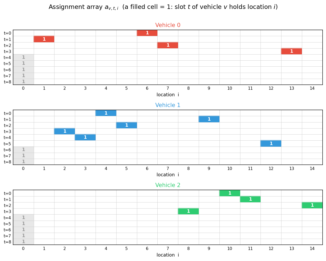
Each vehicle starts at the depot (location 0), visits the customers stored in its non-empty slots in order, and returns to the depot. Each customer $1,\ldots,14$ appears in exactly one slot of exactly one vehicle, so this array represents a feasible CVRP solution. The empty slots line up after the customers, but the formulation does not require this: an empty slot between two customers only means the vehicle passes through the depot in between, which never shortens a route under the triangle inequality. Hence no extra constraint on the position of empty slots is needed, and the optimal solution is naturally a lean set of routes.
Constraints for QUBO++ formulation
Row constraint (one-hot at each slot)
Each slot must hold exactly one location (a customer or the depot for an empty slot). We impose the one-hot constraint:
\[\begin{aligned} \text{row}\_\text{constraint} & = \sum_{v=0}^{V-1}\sum_{t=0}^{L-1}\bigr(\sum_{i=0}^{N-1} a_{v,t,i} = 1\bigl)\\ &= \sum_{v=0}^{V-1}\sum_{t=0}^{L-1}\bigr(1-\sum_{i=0}^{N-1} a_{v,t,i}\bigl)^2 \end{aligned}\]row_constraint attains its minimum value $0$ if and only if every row is one-hot.
Column constraint
Each customer must be held by exactly one slot of exactly one vehicle:
\[\begin{aligned} \text{column}\_\text{constraint} & = \sum_{i=1}^{N-1}\bigr(\sum_{v=0}^{V-1}\sum_{t=0}^{L-1} a_{v,t,i} = 1\bigl)\\ &= \sum_{i=1}^{N-1}\bigr(1-\sum_{v=0}^{V-1}\sum_{t=0}^{L-1} a_{v,t,i}\bigl)^2 \end{aligned}\]column_constraint is 0 if and only if every customer $i = 1, \dots ,N−1$ is visited exactly once. Note that no such constraint is imposed on the depot column $i=0$: any number of slots may be empty.
Capacity constraint
For each vehicle $v$, the total delivered demand is
\[\sum_{t=0}^{L-1}\sum_{i=1}^{N-1}d_ia_{v,t,i},\]which must be at most $q_v$. Then the following constraint must be 0:
\[\begin{aligned} \text{capacity}\_\text{constraint} &= \sum_{v=0}^{V-1}\Bigr(0\leq \sum_{t=0}^{L-1}\sum_{i=1}^{N-1}d_ia_{v,t,i}\leq q_v\Bigl) \end{aligned}\]capacity_constraint is 0 if and only if all vehicles do not exceed their capacity.
Objective for QUBO formulation
The total tour cost of a vehicle consists of the leg from the depot to its first slot, the legs between consecutive slots, and the leg from its last slot back to the depot:
\[\begin{aligned} \text{objective} &= \sum_{v=0}^{V-1}\Bigr(\sum_{i=1}^{N-1}c_{0,i}a_{v,0,i} + \sum_{t=0}^{L-2}\sum_{i=0}^{N-1}\sum_{j=0}^{N-1}c_{i,j}a_{v,t,i}a_{v,t+1,j} + \sum_{i=1}^{N-1}c_{i,0}a_{v,L-1,i}\Bigl) \end{aligned}\]Under the Euclidean metric we have $c_{i,i}=0$, so empty slots at the beginning or the end of a route contribute no extra cost, and when all constraints are satisfied $\text{objective}$ equals the total travel cost of all vehicles.
QUBO formulation for the CVRP
Combining the objective and constraints, we obtain the QUBO:
\[\begin{aligned} f &= \text{objective} + P\cdot \text{cons}(\text{row}\_\text{constraint}+\text{column}\_\text{constraint}+\text{capacity}\_\text{constraint}), \end{aligned}\]where $P$ is the constraint weight. Wrapping the constraint part in qbpp.cons() declares it as constraints; the solver then searches efficiently for solutions satisfying them (see Native Constraints).
PyQBPP program
The following PyQBPP program finds a solution to a randomly generated CVRP instance with $N=15$ locations (a depot and 14 customers) and $V=3$ vehicles, with a time limit of 10 seconds. Distances are the exact Euclidean distances computed with math.sqrt (no rounding); we import the real (double) coefficient frontend pyqbpp.d and build objective in real numbers.
import math
import pyqbpp.d as qbpp

locations = [
    (200, 200, 0),  (330, 320, 38), (17, 390, 25),  (57, 352, 13),
    (79, 233, 95),  (9, 316, 16),   (397, 279, 48), (251, 348, 32),
    (258, 157, 63), (3, 215, 31),   (214, 107, 48), (389, 9, 80),
    (106, 371, 61), (198, 314, 47), (315, 155, 76)]
vehicle_capacity = qbpp.array([200, 250, 300])
N, V = len(locations), len(vehicle_capacity)

def dist(i, j):                      # exact Euclidean distance (double)
    x1, y1 = locations[i][0], locations[i][1]
    x2, y2 = locations[j][0], locations[j][1]
    return math.sqrt((x1 - x2) ** 2 + (y1 - y2) ** 2)

sorted_demands = sorted(locations[i][2] for i in range(1, N))
max_capacity = max(vehicle_capacity[v] for v in range(V))
L, acc = 0, 0
for d in sorted_demands:
    if acc + d > max_capacity: break
    acc += d; L += 1

a = qbpp.var("a", shape=(V, L, N))
row_constraint = qbpp.sum(qbpp.vector_sum(a) == 1)
column_sum = [0 for _ in range(N - 1)]
for v in range(V):
    for t in range(L):
        for i in range(1, N):
            column_sum[i - 1] += a[v][t][i]
column_constraint = 0
for i in range(N - 1):
    column_constraint += (column_sum[i] == 1)
vehicle_load = [0 for _ in range(V)]
capacity_constraint = 0
for v in range(V):
    for t in range(L):
        for i in range(1, N):
            vehicle_load[v] += a[v][t][i] * locations[i][2]
    capacity_constraint += (0 <= vehicle_load[v]) & (qbpp.same <= vehicle_capacity[v])
objective = 0.0
for v in range(V):
    for i in range(1, N):
        objective += dist(0, i) * a[v][0][i]
    for t in range(L - 1):
        for i in range(N):
            for j in range(N):
                if dist(i, j) != 0:
                    objective += dist(i, j) * a[v][t][i] * a[v][t + 1][j]
    for i in range(1, N):
        objective += dist(i, 0) * a[v][L - 1][i]

f = objective + 3000 * qbpp.cons(row_constraint + column_constraint +
                                 capacity_constraint)
f.simplify_as_binary()
sol = qbpp.EasySolver(f).search(time_limit=10.0)
print("violated constraints =", f.cons(sol))
print(f"objective = {sol(objective):.2f}")
for v in range(V):
    load = int(sol(vehicle_load[v]))
    cap = int(vehicle_capacity[v])
    route = f"Vehicle {v} : load = {load} / {cap} : 0 "
    for t in range(L):
        for i in range(1, N):
            if sol(a[v][t][i]) == 1:
                route += f"-> {i}({locations[i][2]}) "; break
    print(route + "-> 0")
The program computes the number of slots L (9 for this instance), defines the array a of $V\times L\times N = 3\times 9\times 15 = 405$ binary variables, and combines the objective and constraint terms with qbpp.cons(): f = objective + 3000 * qbpp.cons(...). The Easy Solver then minimizes f with a time limit of 10 seconds. f.cons(sol) is the number of violated constraints (0 when all are satisfied). As an example, the following results are obtained:
violated constraints = 0
objective = 1821.13
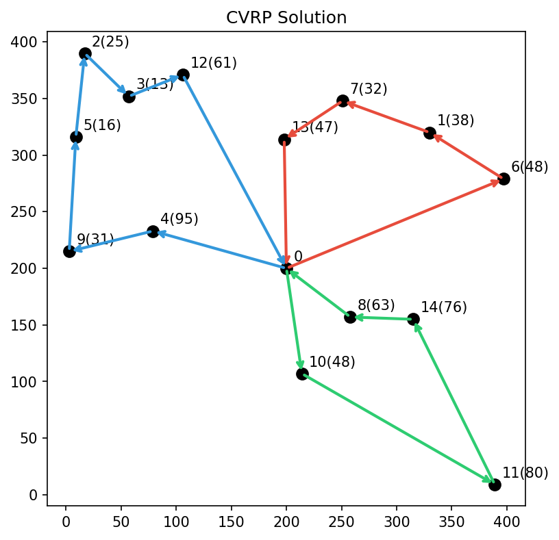
Vehicle 0 : load = 165 / 200 : 0 -> 6(48) -> 1(38) -> 7(32) -> 13(47) -> 0
Vehicle 1 : load = 241 / 250 : 0 -> 4(95) -> 9(31) -> 5(16) -> 2(25) -> 3(13) -> 12(61) -> 0
Vehicle 2 : load = 267 / 300 : 0 -> 10(48) -> 11(80) -> 14(76) -> 8(63) -> 0
The total travel cost of 1821.13 is the best value confirmed by repeated long runs on this instance (we do not prove optimality). Being a heuristic solver, a 10-second run may end slightly above 1821.13 on occasion.
Visualization with matplotlib
The following code visualizes the obtained solution and writes it to cvrp15.png:
import matplotlib.pyplot as plt

vehicle_colors = ["#e74c3c", "#3498db", "#2ecc71"]
plt.figure(figsize=(6, 6))
for i, (lx, ly, q) in enumerate(locations):
    plt.plot(lx, ly, "ko", markersize=8)
    plt.annotate(f"{i}" + (f"({q})" if q > 0 else ""),
                 (lx, ly), textcoords="offset points", xytext=(5, 5))

for v in range(V):
    route_nodes = [0]
    for t in range(L):
        for i in range(1, N):
            if sol(a[v][t][i]) == 1:
                route_nodes.append(i)
                break
    route_nodes.append(0)
    for k in range(len(route_nodes) - 1):
        fr, to = route_nodes[k], route_nodes[k + 1]
        plt.annotate("", xy=(locations[to][0], locations[to][1]),
                     xytext=(locations[fr][0], locations[fr][1]),
                     arrowprops=dict(arrowstyle="->", color=vehicle_colors[v],
                                    lw=2))
plt.title("CVRP Solution")
plt.savefig("cvrp15.png", dpi=150, bbox_inches="tight")
plt.show()
The visualization of the obtained solution (cvrp15.png) is shown below: