Maximum Independent Set (MIS) Problem and Graph Visualization

Graph Visualization in PyQBPP

The C++ version of QUBO++ bundles a simple header-only graph drawing library (qbpp::graph::GraphDrawer) that wraps Graphviz to render graphs directly to svg, png, jpg, or pdf files. See the C++ Graph Library page for details.

PyQBPP does not provide a dedicated graph class. Instead, you can use the widely adopted Python ecosystem for graph visualization:

networkx — graph data structure and layout algorithms
matplotlib — plotting and image export

You can install them with:

pip install networkx matplotlib

The rest of this page explains how to formulate the Maximum Independent Set (MIS) problem as a QUBO, solve it with PyQBPP, and then visualize the resulting graph with networkx + matplotlib.

WARNING: The visualization code shown below is intended for illustrating results produced by PyQBPP sample programs. It relies on third-party libraries whose APIs may change, and it is not recommended for use in mission-critical applications.

Maximum Independent Set (MIS) Problem

An independent set of an undirected graph $G=(V,E)$ is a subset of vertices $S\subseteq V$ such that no two vertices in $S$ are connected by an edge in $E$. The Maximum Independent Set (MIS) problem asks for an independent set with maximum cardinality.

The MIS problem can be formulated as a QUBO as follows. Assume that $G$ has $n$ vertices indexed from $0$ to $n-1$. We introduce $n$ binary variables $x_i$ $(0\le i\le n-1)$, where $x_i=1$ if and only if vertex $i$ is included in $S$. Since we want to maximize $|S|=\sum_{i=0}^{n-1}x_i$, we minimize the following objective:

\[\begin{aligned} \text{objective} = -\sum_{i=0}^{n-1} x_i . \end{aligned}\]

To enforce independence, for every edge $(i,j)\in E$ we must not select both endpoints simultaneously. This can be penalized by

\[\begin{aligned} \text{constraint} = \sum_{(i,j)\in E} x_i x_j . \end{aligned}\]

Combining the objective and the penalty yields the QUBO function

\[\begin{aligned} f = \text{objective} + 2\times\text{constraint}. \end{aligned}\]

The penalty coefficient $2$ is sufficient to prioritize feasibility over increasing the set size.

PyQBPP Program for the MIS Problem

Based on the QUBO formulation of the MIS problem described above, the following PyQBPP program solves an instance with 16 nodes. The edges are stored in edges:

import pyqbpp as qbpp

N = 16
edges = [
    (0, 1),  (0, 2),  (1, 3),  (1, 4),  (2, 5),  (2, 6),
    (3, 7),  (3, 13), (4, 6),  (4, 7),  (5, 8),  (6, 8),
    (6, 14), (7, 14), (8, 9),  (9, 10), (9, 12), (10, 11),
    (10, 12),(11, 13),(12, 14),(13, 15),(14, 15)]

x = qbpp.var("x", shape=N)

objective = -qbpp.sum(x)
constraint = qbpp.expr()
for u, v in edges:
    constraint += x[u] * x[v]
f = objective + constraint * 2
f.simplify_as_binary()

solver = qbpp.ExhaustiveSolver(f)
sol = solver.search()

print(f"objective = {sol(objective)}")
print(f"constraint = {sol(constraint)}")

print("Selected nodes:", end="")
for i in range(N):
    if sol(x[i]) == 1:
        print(f" {i}", end="")
print()

For a vector x of N = 16 binary variables created by qbpp.var("x", shape=N), the expressions objective, constraint, and f are constructed according to the above QUBO formulation. Here qbpp.expr() creates a zero expression that serves as an accumulator for the penalty sum over the edges, and qbpp.sum(x) sums all entries of x. The QUBO function f is then simplified in place via f.simplify_as_binary(), which applies the binary (0/1) rule to merge like terms.

The Exhaustive Solver is then used to find an optimal solution for f, which is stored in sol. The values of objective and constraint evaluated at sol are obtained via sol(objective) and sol(constraint) and printed. Finally, the list of selected nodes is printed by iterating over the indices i and checking whether sol(x[i]) == 1, which evaluates the binary variable x[i] at the solution.

This program produces the following output:

objective = -7
constraint = 0
Selected nodes: 0 4 5 9 11 13 14

This implies that the obtained solution selects 7 nodes and satisfies all constraints.

Visualization using matplotlib and networkx

The following code visualizes the MIS solution. Append it to the program above so that edges, N, x, and sol are still in scope:

import matplotlib.pyplot as plt
import networkx as nx

G = nx.Graph()
G.add_nodes_from(range(N))
G.add_edges_from(edges)
pos = nx.spring_layout(G, seed=42)

colors = ["#e74c3c" if sol(x[i]) == 1 else "#d5dbdb" for i in range(N)]
nx.draw(G, pos, with_labels=True, node_color=colors, node_size=400,
        font_size=9, edge_color="#888888", width=1.2)
plt.title("Maximum Independent Set")
plt.savefig("mis.png", dpi=150, bbox_inches="tight")
plt.show()

A networkx.Graph object G is created, and the nodes and edges are added using add_nodes_from() and add_edges_from(). The layout positions pos are computed with the spring-layout algorithm (with a fixed seed for reproducibility).

A color list colors is built from the solver output: selected nodes (sol(x[i]) == 1) are drawn in red (#e74c3c), while unselected nodes are drawn in light gray (#d5dbdb). nx.draw() renders the graph with node labels enabled, and plt.savefig() writes the resulting image to mis.png. The output format is determined by the file extension, so passing "mis.svg" or "mis.pdf" instead of "mis.png" produces the corresponding format.

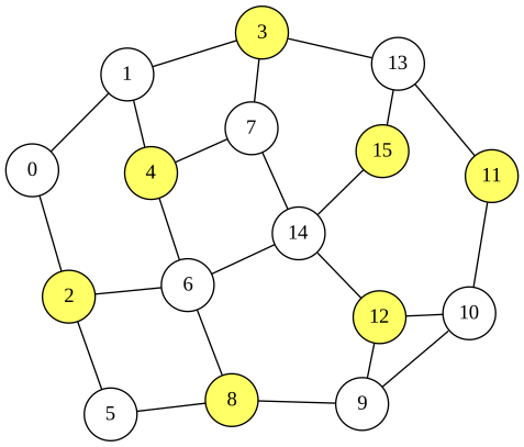
The rendered image is similar to the one below (which is produced by the C++ version using qbpp::graph::GraphDrawer). Note that the exact node placement may differ because networkx.spring_layout uses a force-directed algorithm while the C++ library relies on Graphviz’s neato:

The solution of the MIS problem.

Mapping from the C++ Graph Library

The table below summarizes how the C++ graph drawing API maps to the Python ecosystem:

C++ (`qbpp/graph.hpp`)	Python equivalent
`qbpp::graph::Node(i)`	`G.add_node(i)` on a `networkx.Graph`
`Node::color(int)` / `color(str)`	`node_color=[...]` argument of `nx.draw()`
`Node::position(x, y)`	Entry in the `pos` dict passed to `nx.draw()`
`Node::penwidth(f)`	`linewidths=...` argument of `nx.draw()`
`qbpp::graph::Edge(u, v)`	`G.add_edge(u, v)` on a `networkx.Graph`
`Edge::directed()`	Use `networkx.DiGraph` instead of `Graph`
`Edge::color(...)`	`edge_color=[...]` argument of `nx.draw()`
`Edge::penwidth(f)`	`width=...` argument of `nx.draw()`
`GraphDrawer::add_node/edge`	`G.add_node` / `G.add_edge`
`GraphDrawer::write("f.svg")`	`plt.savefig("f.svg")` (or `.png`, `.pdf`, `.jpg`)

NOTE: PyQBPP intentionally does not reimplement the C++ graph drawing helper. networkx + matplotlib offers a richer, well-maintained ecosystem for Python users, and the resulting images are equivalent for visualizing solver output from QUBO formulations.