Image Halftoning
Halftoning converts a grayscale image into a binary (black-and-white) dot-pattern image. It is used to reproduce continuous tones on media that can only display two levels, such as newspaper photographs and monochrome printers. Viewed from a distance, the fine black-and-white pattern is averaged by the eye and perceived as intermediate tones.
This “blurring in the eye” is the key to the formulation. If we model the blur of the human visual system by a low-pass (Gaussian) filter $G$, a good halftone image is a binary image whose
blurred version is as close as possible to the original image.
Minimizing the sum of squared differences is directly a QUBO problem, with no auxiliary variables and no constraints.
QUBO Formulation
Suppose an $n_r \times n_c$ grayscale image $I$ (pixel values $0 \le I_{ij} \le 255$) is given. We assign a binary variable $x_{ij} \in {0,1}$ to every output pixel ($1$ = white, $0$ = black), so the number of variables equals the number of pixels, $n_r n_c$.
The blur is a convolution with a $(2M{+}1)\times(2M{+}1)$ filter $G$ (the example below uses $M=3$ and a $7\times 7$ integer Gaussian whose coefficients sum to $255$). The blur of the binary image $x$ is
\[(G * x)_{ij} = \sum_{k=0}^{2M} \sum_{l=0}^{2M} G_{kl}\, x_{i+k-M,\, j+l-M}\]where pixels outside the image are treated as $0$. Because the coefficients of $G$ sum to $255$, each element of $(G * x)$ ranges over $0$–$255$ in the interior of the image. The target is the original image itself:
\[T_{ij} = \mathrm{round}\!\left(\frac{I_{ij}\, m_{ij}}{255}\right), \qquad m_{ij} = (G * \mathbf{1})_{ij}\]where $m_{ij}$ is the total filter mass reaching pixel $(i,j)$ ($\mathbf{1}$ is the all-ones image). In the interior $m_{ij} = 255$, so $T_{ij} = I_{ij}$ — the original image as is. Near the border the filter window sticks out of the image and the maximum value the blur can reach at that pixel drops to $m_{ij}$, so the target is scaled down by the same ratio.
One could instead use a blurred version of the original image as the target, but using the unblurred original produces a sharper halftone image that looks better to the human eye.
The objective function to minimize is the sum of squared differences between the blurred binary image and the target:
\[E(x) = \sum_{i,j} \bigl( (G * x)_{ij} - T_{ij} \bigr)^2\]Each element of $(G * x)$ is a linear expression in the variables, so $E(x)$ is quadratic — a pure, unconstrained QUBO. A product of two variables $x_{ij}\, x_{kl}$ appears in the expansion of the squares only if the two pixels $(i,j)$ and $(k,l)$ share a filter window, i.e., their vertical and horizontal distances are at most $2M$, so the QUBO is sparse (band structure).
PyQBPP Program
The following program generates a $64\times 64$ synthetic grayscale image (a diagonal gradient plus a bright disk), halftones it, and saves the result as an image file in PGM format:
import pyqbpp as qbpp

M = 3                                        # filter radius (7x7 filter)
G = [[0, 0, 1, 1, 1, 0, 0],
     [0, 1, 5, 7, 5, 1, 0],
     [1, 5, 14, 21, 14, 5, 1],
     [1, 7, 21, 31, 21, 7, 1],
     [1, 5, 14, 21, 14, 5, 1],
     [0, 1, 5, 7, 5, 1, 0],
     [0, 0, 1, 1, 1, 0, 0]]                  # integer Gaussian (sum = 255)
ROWS = COLS = 64

def blur(a):
    # convolution with G (pixels outside the image are treated as 0)
    out = [[0] * COLS for _ in range(ROWS)]
    for i in range(ROWS):
        for j in range(COLS):
            for k in range(2 * M + 1):
                for l in range(2 * M + 1):
                    if 0 <= i + k - M < ROWS and 0 <= j + l - M < COLS:
                        out[i][j] += G[k][l] * a[i + k - M][j + l - M]
    return out

# input image: diagonal gradient + bright disk (synthetic)
img = [[235 if (i - 20) ** 2 + (j - 44) ** 2 < 196
        else 255 * (i + j) // (ROWS + COLS - 2) for j in range(COLS)]
       for i in range(ROWS)]

# target T: the original image itself (scaled near the border
# by the reachable filter mass)
mass = blur([[1] * COLS for _ in range(ROWS)])
target = [[round(img[i][j] * mass[i][j] / 255) for j in range(COLS)]
          for i in range(ROWS)]

# E = sum(((G * x) - T)^2): build (G * x) - T pixel by pixel, sum the squares
x = qbpp.var("x", ROWS, COLS)
f = 0
for i in range(ROWS):
    for j in range(COLS):
        e = 0
        for k in range(2 * M + 1):
            for l in range(2 * M + 1):
                if 0 <= i + k - M < ROWS and 0 <= j + l - M < COLS and G[k][l]:
                    e += G[k][l] * x[i + k - M, j + l - M]
        f += qbpp.sqr(e - target[i][j])
f.simplify_as_binary()

sol = qbpp.EasySolver(f).search(time_limit=5)
print("variables =", sol.info["var_count"], " terms =", sol.info["term_count"])
print("energy =", sol.energy)

# save the solution as a binary image in PGM format
bits = sol(x)
with open("halftone.pgm", "w") as fp:
    fp.write(f"P2\n{COLS} {ROWS}\n255\n")
    for i in range(ROWS):
        fp.write(" ".join(str(255 * int(v)) for v in bits[i]) + "\n")
The inner double loop builds, for every pixel, the blur value $(G * x)$ minus the target, squares it with qbpp.sqr, and accumulates it into f — a direct transcription of the formula. simplify_as_binary() merges like terms and applies the binary-variable rule $x^2 = x$.
Output
variables = 4096  terms = 244488
energy = 259375
With $64\times 64$ pixels there are $4096$ variables, and the simplified QUBO has about $240{,}000$ terms (a band structure in which each variable interacts only with neighbors within $\pm 2M$ vertically and horizontally). Since EasySolver is a randomized heuristic, the energy varies from run to run.
The input image (left) and the resulting halftone image (right):
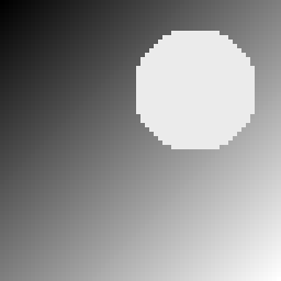
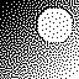
The gradient is reproduced as a varying density of white dots.
Vectorizing the Construction with Array Operations
The double loop that builds f can be vectorized with QUBO++ array operations (x is used as is):
# zero padding: concatenate zeros of width M around x
xp = qbpp.concat([0] * M + [x] + [0] * M, axis=1)   # left/right
xp = qbpp.concat([0] * M + [xp] + [0] * M, axis=0)  # top/bottom

# (G * x): weighted sum of shifted slices
conv = qbpp.expr(ROWS, COLS)
for k in range(2 * M + 1):
    for l in range(2 * M + 1):
        if G[k][l]:
            conv += G[k][l] * xp[k:k + ROWS, l:l + COLS]

# E = sum(((G * x) - T)^2)
f = qbpp.sum((conv - qbpp.array(target)).sqr())
f.simplify_as_binary()
qbpp.concatconcatenates zeros of width $M$ aroundx, producing the padded $(n_r{+}2M) \times (n_c{+}2M)$ arrayxp(a scalar0in the list is automatically broadcast to a zero row/column along the concatenation axis).- The $n_r \times n_c$ subarray of
xpshifted by $k, l$, i.e.,xp[k:k + ROWS, l:l + COLS], is multiplied by the coefficient $G_{kl}$ and accumulated intoconv. After this double loop,convis the array of linear expressions $(G * x)$. - Subtracting the target array
qbpp.array(target), squaring elementwise withsqr(), and summing withqbpp.sumyields the objective function $E(x)$.
Both versions build exactly the same QUBO (the term count after simplify and the energies agree exactly). The construction time, however, is about 2–2.5 times shorter with array operations (measured on a 20-core CPU server):
| Image size | Loop | Array operations |
|---|---|---|
| 64×64 | 1.3 s | 0.6 s |
| 128×128 | 3.7 s | 1.8 s |
| 256×256 | 14.8 s | 6.0 s |
Note that the loop accumulation must be written as f += .... Writing f = f + ... instead copies the whole of f for every pixel and slows down quadratically (about 80 times slower at 64×64 in our measurement).
The loop version repeats a small expression operation per pixel and per tap (millions of calls at 256×256), while the array version issues a few dozen coarse-grained array operations whose element-wise work runs inside the library.
Applying to Real Images
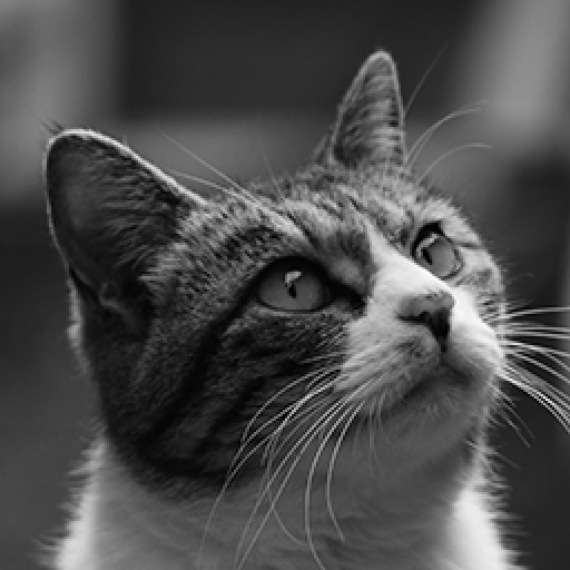
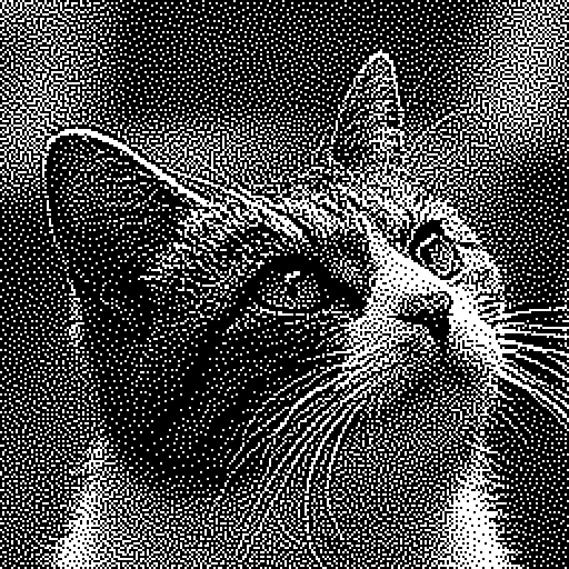
Replacing the image-generation part with file input lets you halftone real photographs. A $256\times 256$ photograph yields a QUBO with $65{,}536$ variables and about $4.17$ million terms, but building it takes only a few seconds, and a few minutes of EasySolver search produce the following result: