Permutation matrix generation

Many combinatorial optimization problems are permutation-based in the sense that the objective is to find an optimal permutation. As a fundamental technique for formulating such optimization problems, a matrix of binary variables is used in their QUBO formulation.

Permutation matrix

Let $X=(x_{i,j})$ ($0\leq i,j\leq n-1$) is a matrix of $n\times n$ binary values. The matrix $X$ is called a permutation matrix if and only if every row and every column has exactly one entry equal to 1, as shown below.

Permutation matrix

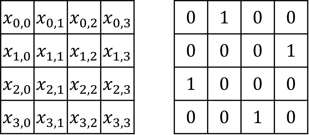
A permutation matrix represents a permutation of $n$ numbers $(0,1,\ldots,n-1)$, where $x_{i,j} = 1$ if and only if the $i$-th element is $j$. For example, the above permutation matrix represents the permutation $(1,3,0,2)$.

QUBO formulation for permutation matrices

A binary variable matrix $X=(x_{i,j})$ ($0\leq i,j\leq n-1$) stores a permutation matrix if and only if the sum of each row and each column is 1. Thus, the following QUBO function takes the minimum value 0 if and only if $X$ stores a permutation matrix:

\[\begin{aligned} f(X) &= \sum_{i=0}^{n-1}\left(1-\sum_{j=0}^{n-1}x_{i,j}\right)^2+\sum_{j=0}^{n-1}\left(1-\sum_{i=0}^{n-1}x_{i,j}\right)^2 \end{aligned}\]

PyQBPP program for generating permutation matrices

A two-dimensional array of binary variables is created by passing a tuple to the shape= keyword argument. For example, qbpp.var("x", shape=(4, 4)) returns a $4\times 4$ array of binary variables, with each element accessed as x[i][j]. Higher-dimensional arrays are created in the same way — e.g. shape=(2, 3, 4) for a 3D array. See Multi-dimensional Variables for details.

We can design a PyQBPP program based on the formula $f(X)$ above as follows:

import pyqbpp as qbpp

x = qbpp.var("x", shape=(4, 4))
f = qbpp.expr()

for i in range(4):
    s = qbpp.expr()
    for j in range(4):
        s += x[i][j]
    f += qbpp.sqr(1 - s)

for j in range(4):
    s = qbpp.expr()
    for i in range(4):
        s += x[i][j]
    f += qbpp.sqr(1 - s)

f.simplify_as_binary()
solver = qbpp.ExhaustiveSolver(f)
result = solver.search(best_energy_sols=0)
for k, sol in enumerate(result.sols):
    print(f"Solution {k} : {sol(x)}")

In this program, qbpp.var("x", shape=(4, 4)) returns an array object of shape ${4, 4}$ named x. For an Expr object f, two double for-loops add the formulas for $f(X)$. Using the Exhaustive Solver, all optimal solutions are computed and stored in result.sols. All solutions in result.sols are displayed one-by-one. Here, sol(x) returns a matrix of values of x in sol (an array of int). This program outputs all 24 permutations as follows:

Solution 0 : [[0, 0, 0, 1], [0, 0, 1, 0], [0, 1, 0, 0], [1, 0, 0, 0]]
Solution 1 : [[0, 0, 0, 1], [0, 0, 1, 0], [1, 0, 0, 0], [0, 1, 0, 0]]
Solution 2 : [[0, 0, 0, 1], [0, 1, 0, 0], [0, 0, 1, 0], [1, 0, 0, 0]]
Solution 3 : [[0, 0, 0, 1], [0, 1, 0, 0], [1, 0, 0, 0], [0, 0, 1, 0]]
Solution 4 : [[0, 0, 0, 1], [1, 0, 0, 0], [0, 0, 1, 0], [0, 1, 0, 0]]
Solution 5 : [[0, 0, 0, 1], [1, 0, 0, 0], [0, 1, 0, 0], [0, 0, 1, 0]]
Solution 6 : [[0, 0, 1, 0], [0, 0, 0, 1], [0, 1, 0, 0], [1, 0, 0, 0]]
Solution 7 : [[0, 0, 1, 0], [0, 0, 0, 1], [1, 0, 0, 0], [0, 1, 0, 0]]
Solution 8 : [[0, 0, 1, 0], [0, 1, 0, 0], [0, 0, 0, 1], [1, 0, 0, 0]]
Solution 9 : [[0, 0, 1, 0], [0, 1, 0, 0], [1, 0, 0, 0], [0, 0, 0, 1]]
Solution 10 : [[0, 0, 1, 0], [1, 0, 0, 0], [0, 0, 0, 1], [0, 1, 0, 0]]
Solution 11 : [[0, 0, 1, 0], [1, 0, 0, 0], [0, 1, 0, 0], [0, 0, 0, 1]]
Solution 12 : [[0, 1, 0, 0], [0, 0, 0, 1], [0, 0, 1, 0], [1, 0, 0, 0]]
Solution 13 : [[0, 1, 0, 0], [0, 0, 0, 1], [1, 0, 0, 0], [0, 0, 1, 0]]
Solution 14 : [[0, 1, 0, 0], [0, 0, 1, 0], [0, 0, 0, 1], [1, 0, 0, 0]]
Solution 15 : [[0, 1, 0, 0], [0, 0, 1, 0], [1, 0, 0, 0], [0, 0, 0, 1]]
Solution 16 : [[0, 1, 0, 0], [1, 0, 0, 0], [0, 0, 0, 1], [0, 0, 1, 0]]
Solution 17 : [[0, 1, 0, 0], [1, 0, 0, 0], [0, 0, 1, 0], [0, 0, 0, 1]]
Solution 18 : [[1, 0, 0, 0], [0, 0, 0, 1], [0, 0, 1, 0], [0, 1, 0, 0]]
Solution 19 : [[1, 0, 0, 0], [0, 0, 0, 1], [0, 1, 0, 0], [0, 0, 1, 0]]
Solution 20 : [[1, 0, 0, 0], [0, 0, 1, 0], [0, 0, 0, 1], [0, 1, 0, 0]]
Solution 21 : [[1, 0, 0, 0], [0, 0, 1, 0], [0, 1, 0, 0], [0, 0, 0, 1]]
Solution 22 : [[1, 0, 0, 0], [0, 1, 0, 0], [0, 0, 0, 1], [0, 0, 1, 0]]
Solution 23 : [[1, 0, 0, 0], [0, 1, 0, 0], [0, 0, 1, 0], [0, 0, 0, 1]]

NOTE A matrix of binary variables is implemented as a multi-dimensional array using the array class. For example, qbpp.var("x", shape=(4, 4)) returns an array object with shape (4, 4). Each Var object is represented as x[i][j] and the value of x[i][j] for sol can be obtained by either sol(x[i][j]) or x[i][j](sol).

QUBO formulation for a permutation matrix using array functions and operations

Using qbpp.vector_sum(), we can compute the row-wise and column-wise sums of a matrix x of binary variables:

qbpp.vector_sum(x, axis=1): Computes the sum of each row of x and returns an array of size n containing these sums.
qbpp.vector_sum(x, axis=0): Computes the sum of each column of x and returns an array of size n containing these sums.

Note: For a multi-dimensional array x and an axis k, qbpp.vector_sum(x, axis=k) computes sums along axis k and returns a multi-dimensional array whose dimension is reduced by one. For a 2-dimensional array (matrix) x, axis 1 corresponds to the row direction, and axis 0 corresponds to the column direction.

A scalar-array operation can be used to subtract 1 from each element:

qbpp.vector_sum(x, axis=1) - 1: subtracts 1 from each row-wise sum.
qbpp.vector_sum(x, axis=0) - 1: subtracts 1 from each column-wise sum.

For these two arrays of size n, qbpp.sqr() squares each element, and qbpp.sum() computes the sum of all elements.

The following PyQBPP program implements a QUBO formulation using these array functions and operations:

import pyqbpp as qbpp

x = qbpp.var("x", shape=(4, 4))
f = qbpp.sum(qbpp.sqr(qbpp.vector_sum(x, axis=1) - 1)) + \
    qbpp.sum(qbpp.sqr(qbpp.vector_sum(x, axis=0) - 1))
f.simplify_as_binary()

solver = qbpp.ExhaustiveSolver(f)
result = solver.search(best_energy_sols=0)
for k, sol in enumerate(result.sols):
    row = qbpp.onehot_to_int(sol(x), axis=1)
    column = qbpp.onehot_to_int(sol(x), axis=0)
    print(f"Solution {k}: {row}, {column}")

In this program, sol(x) returns a matrix of assigned values to x in sol, which is a matrix of integer values with the same shape as x. qbpp.onehot_to_int() converts one-hot arrays along the axis to the corresponding integers.

qbpp.onehot_to_int(sol(x), axis=1): Computes the integer corresponding to each row and returns them as an array of 4 integers, which represents the permutation.
qbpp.onehot_to_int(sol(x), axis=0): returns the integer corresponding to each column and returns them as an array of 4 integers, which represents the inverse of the permutation.

This program outputs all permutations and their inverse as integer vectors as follows:

Solution 0: [3, 2, 1, 0], [3, 2, 1, 0]
Solution 1: [3, 2, 0, 1], [2, 3, 1, 0]
Solution 2: [3, 1, 2, 0], [3, 1, 2, 0]
Solution 3: [3, 1, 0, 2], [2, 1, 3, 0]
Solution 4: [3, 0, 2, 1], [1, 3, 2, 0]
Solution 5: [3, 0, 1, 2], [1, 2, 3, 0]
Solution 6: [2, 3, 1, 0], [3, 2, 0, 1]
Solution 7: [2, 3, 0, 1], [2, 3, 0, 1]
Solution 8: [2, 1, 3, 0], [3, 1, 0, 2]
Solution 9: [2, 1, 0, 3], [2, 1, 0, 3]
Solution 10: [2, 0, 3, 1], [1, 3, 0, 2]
Solution 11: [2, 0, 1, 3], [1, 2, 0, 3]
Solution 12: [1, 3, 2, 0], [3, 0, 2, 1]
Solution 13: [1, 3, 0, 2], [2, 0, 3, 1]
Solution 14: [1, 2, 3, 0], [3, 0, 1, 2]
Solution 15: [1, 2, 0, 3], [2, 0, 1, 3]
Solution 16: [1, 0, 3, 2], [1, 0, 3, 2]
Solution 17: [1, 0, 2, 3], [1, 0, 2, 3]
Solution 18: [0, 3, 2, 1], [0, 3, 2, 1]
Solution 19: [0, 3, 1, 2], [0, 2, 3, 1]
Solution 20: [0, 2, 3, 1], [0, 3, 1, 2]
Solution 21: [0, 2, 1, 3], [0, 2, 1, 3]
Solution 22: [0, 1, 3, 2], [0, 1, 3, 2]
Solution 23: [0, 1, 2, 3], [0, 1, 2, 3]

Assignment problem and its QUBO formulation

Let $C = (c_{i,j})$ be a cost matrix of size $n \times n$. The assignment problem for $C$ is to find a permutation $p:\lbrace 0,1,\ldots, n-1\rbrace \rightarrow \lbrace 0,1,\ldots, n-1\rbrace$ that minimizes the total cost:

\[\begin{aligned} g(p) &= \sum_{i=0}^{n-1}c_{i,p(i)} \end{aligned}\]

We can use a permutation matrix $X = (x_{i,j})$ of size $n \times n$ for a QUBO formulation of this problem by defining:

\[\begin{aligned} g(X) &= \sum_{i=0}^{n-1}\sum_{j=0}^{n-1}c_{i,j}x_{i,j} \end{aligned}\]

Clearly, $g(p) = g(X)$ holds if and only if $X$ represents the permutation $p$.

We combine the QUBO formulation for the permutation matrix, $f(X)$, and the total cost, $g(X)$, to obtain a QUBO formulation of the assignment problem:

\[\begin{aligned} h(X) &= P\cdot f(X)+g(X) \\ &=P\left(\sum_{i=0}^{n-1}\left(1-\sum_{j=0}^{n-1}x_{i,j}\right)^2+\sum_{j=0}^{n-1}\left(1-\sum_{i=0}^{n-1}x_{i,j}\right)^2\right)+\sum_{i=0}^{n-1}\sum_{j=0}^{n-1}c_{i,j}x_{i,j} \end{aligned}\]

Here, $P$ is a sufficiently large positive constant that prioritizes the permutation constraints encoded in $f(X)$.

PyQBPP program for the assignment problem

We are now ready to design a PyQBPP program for the assignment problem. In this program, a fixed matrix $C$ of size $4\times4$ is given as an array. qbpp.array() automatically converts nested Python lists into nested array objects, so multi-dimensional arrays can be created concisely. The formulas for $f(X)$ and $g(X)$ are defined using array functions and operations. Here, qbpp.constrain(qbpp.vector_sum(x, axis=1), equal=1) returns an array of QUBO expressions that take the minimum value 0 when the equality vector_sum(x, axis=1) == 1 is satisfied. In fact, it returns the same QUBO expressions as qbpp.sqr(qbpp.vector_sum(x, axis=1) - 1). Also, c * x returns a matrix obtained by computing the element-wise product of c and x, and therefore qbpp.sum(c * x) returns g(X).

import pyqbpp as qbpp

c = qbpp.array([[58, 73, 91, 44],
                [62, 15, 87, 39],
                [78, 56, 23, 94],
                [11, 85, 68, 72]])
x = qbpp.var("x", shape=(4, 4))
f = qbpp.sum(qbpp.constrain(qbpp.vector_sum(x, axis=1), equal=1)) + \
    qbpp.sum(qbpp.constrain(qbpp.vector_sum(x, axis=0), equal=1))
g = qbpp.sum(c * x)
h = 1000 * f + g
h.simplify_as_binary()

solver = qbpp.EasySolver(h)
sol = solver.search(time_limit=1.0)
print("sol =", sol)
result = qbpp.onehot_to_int(sol(x), axis=1)
print("Result :", result)
for i in range(len(result)):
    print(f"c[{i}][{result[i]}] = {c[i][result[i]]}")

We use the Easy Solver to find a solution of h. For an Easy Solver object solver for h, the time limit for searching a solution is set to 1.0 seconds by passing time_limit=1.0 to search(). The resulting permutation is stored in result, and the selected c[i][j] values are printed in turn. The output of this program is as follows:

sol = 93:{x[0][0]: 0, x[0][1]: 0, x[0][2]: 0, x[0][3]: 1, x[1][0]: 0, x[1][1]: 1, x[1][2]: 0, x[1][3]: 0, x[2][0]: 0, x[2][1]: 0, x[2][2]: 1, x[2][3]: 0, x[3][0]: 1, x[3][1]: 0, x[3][2]: 0, x[3][3]: 0}
Result : [3, 1, 2, 0]
c[0][3] = 44
c[1][1] = 15
c[2][2] = 23
c[3][0] = 11

NOTE For an expression f and an integer m, qbpp.constrain(f, equal=m) returns an expression sqr(f - m), which takes the minimum value 0 if and only if the equality f == m is satisfied.

Writing the assignment problem with native constraints `cons()`

In the program above, the permutation constraint f was added to the objective as a penalty expression with weight 1000. PyQBPP lets you explicitly declare the one-hot constraints on the rows and columns by wrapping them in qbpp.cons():

import pyqbpp as qbpp

c = qbpp.array([[58, 73, 91, 44],
                [62, 15, 87, 39],
                [78, 56, 23, 94],
                [11, 85, 68, 72]])
x = qbpp.var("x", shape=(4, 4))
g = qbpp.sum(c * x)
h = g + 1000 * (qbpp.cons(qbpp.vector_sum(x, axis=1) == 1) +
                qbpp.cons(qbpp.vector_sum(x, axis=0) == 1))
h.simplify_as_binary()

solver = qbpp.EasySolver(h)
sol = solver.search(time_limit=1.0)
result = qbpp.onehot_to_int(sol(x), axis=1)
print("Result :", result)
print("violated constraints =", h.cons(sol))
for i in range(len(result)):
    print(f"c[{i}][{result[i]}] = {c[i][result[i]]}")

When an array comparison such as qbpp.vector_sum(x, axis=1) == 1 is wrapped in qbpp.cons(), it is declared as one constraint per element (here, one per row and one per column). The declared constraints are treated specially as constraints, and the bundled solvers search efficiently for a permutation matrix that satisfies them. h.cons(sol) returns the number of constraints violated by the solution sol (0 means x is a permutation matrix). The output of this program is as follows:

Result : [3, 1, 2, 0]
violated constraints = 0
c[0][3] = 44
c[1][1] = 15
c[2][2] = 23
c[3][0] = 11

See Native Constraints for more about cons().

Permutation matrix generation