Simulating a Quantum Annealer

A quantum annealer is a device that searches for spin assignments with low Ising model energy on a graph whose couplings between qubits are fixed by the hardware. If you write the same Ising model as a PyQBPP expression and solve it, you obtain the solution the quantum annealer is expected to return. In other words, you can simulate a quantum annealer without using the real machine. This is useful for checking a program before sending a problem to the machine, and for comparing the solutions the machine returns with the optimum.

On this page, we solve an Ising model with random coefficients, in the same ranges as the real machine, on the Chimera graph, which is the coupling layout of the D-Wave 2000Q quantum annealer. The 2000Q is no longer available, and the current D-Wave quantum annealer is Advantage2. We use the Chimera graph of the 2000Q because its structure is easy to understand, but the same approach works for Advantage2 (see Advantage2).

Ising model

Qubit $i$ represents a spin $s_i\in\lbrace -1,+1\rbrace$. Let $E$ be the set of edges of the graph whose nodes are the qubits and whose edges are the couplings. The energy of the Ising model is:

\[E(s) = \sum_{i} h_i s_i + \sum_{(i,j)\in E} J_{ij}\, s_i s_j\]

$h_i$ is the field on qubit $i$ and $J_{ij}$ is the strength of the coupling between qubits $i$ and $j$; both are real numbers. A coupling with $J_{ij}<0$ lowers the energy when $s_i$ and $s_j$ are equal, and a coupling with $J_{ij}>0$ lowers it when they differ. The user gives $h_i$ and $J_{ij}$, and the quantum annealer returns spin assignments with low $E(s)$. On the 2000Q, the allowed ranges are $-2\le h_i\le 2$ and $-1\le J_{ij}\le 1$.

Chimera graph

The qubits of the 2000Q are coupled in the form of a Chimera graph. A Chimera graph is a grid of cells, each of which has 8 qubits. The 8 qubits of a cell are split into two groups of 4 (group 0 and group 1), coupled as follows:

Inside a cell, each qubit of group 0 is coupled to all 4 qubits of group 1.
Each qubit of group 0 is coupled to the qubit at the same position in group 0 of the cell below.
Each qubit of group 1 is coupled to the qubit at the same position in group 1 of the cell to the right.

The 2000Q had 16×16 cells (2048 qubits). On this page, we use 2×2 cells (32 qubits and 80 couplings):

Chimera graph with 2×2 cells

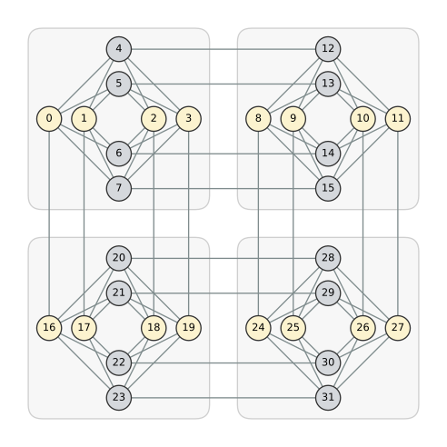
The light gray squares are the cells; the 4 yellow qubits are group 0 and the 4 gray qubits are group 1. Group 0 is drawn as a horizontal row and is coupled to the cell below by vertical edges. Group 1 is drawn as a vertical column and is coupled to the cell to the right by horizontal edges.

The $k$-th qubit ($k=0,1,2,3$) of group $u$ in the cell at row $i$ and column $j$ gets the number $((i\cdot C+j)\cdot 2+u)\cdot 4+k$, where $C$ is the number of cell columns. This numbering is the same as that of the Chimera graphs generated by D-Wave’s Ocean SDK.

Converting to QUBO

PyQBPP solvers solve expressions of binary variables, which take the value 0 or 1. If we relate a spin $s_i$ and a binary variable $x_i$ by $s_i=2x_i-1$ ($s_i=+1$ when $x_i=1$ and $s_i=-1$ when $x_i=0$), $E(s)$ becomes an expression of binary variables. In PyQBPP, you can write $E(s)$ with spin variables and call spin_to_binary() to make this substitution. The substituted expression has the same value as the original $E(s)$, so the energy returned by the solver is exactly the energy of the Ising model.

PyQBPP program

The following PyQBPP program solves the Ising model with random coefficients on the Chimera graph with 2×2 cells:

import random
import pyqbpp.d as qbpp


def chimera(rows, cols):
    L = 4  # number of qubits in each group of a cell

    def q(i, j, u, k):
        return ((i * cols + j) * 2 + u) * L + k

    nodes = list(range(rows * cols * 2 * L))
    edges = []
    for i in range(rows):
        for j in range(cols):
            for k in range(L):
                for l in range(L):
                    edges.append((q(i, j, 0, k), q(i, j, 1, l)))
                if i + 1 < rows:
                    edges.append((q(i, j, 0, k), q(i + 1, j, 0, k)))
                if j + 1 < cols:
                    edges.append((q(i, j, 1, k), q(i, j + 1, 1, k)))
    return nodes, edges


ROWS, COLS = 2, 2  # numbers of cell rows and columns
nodes, edges = chimera(ROWS, COLS)

random.seed(1)
h = {v: random.uniform(-2, 2) for v in nodes}
J = {e: random.uniform(-1, 1) for e in edges}

s = qbpp.var("s", shape=len(nodes))
f = 0
for v in nodes:
    f += h[v] * s[v]
for (a, b), w in J.items():
    f += w * s[a] * s[b]
f.spin_to_binary()
f.simplify_as_binary()

solver = qbpp.EasySolver(f)
sol = solver.search(time_limit=1)

spin = {v: 2 * sol(s[v]) - 1 for v in nodes}
E = 0
for v in nodes:
    E += h[v] * spin[v]
for (a, b), w in J.items():
    E += w * spin[a] * spin[b]
print(f"energy = {sol.energy:.4f}")
print(f"E(s)   = {E:.4f}")
for i in range(ROWS):
    for j in range(COLS):
        v = (i * COLS + j) * 8
        left = " ".join(f"{spin[v + k]:+d}" for k in range(4))
        right = " ".join(f"{spin[v + k]:+d}" for k in range(4, 8))
        print(f"cell ({i},{j}): {left} | {right}")

This program does the following:

import pyqbpp.d makes the coefficients of expressions real numbers (float) (see Real (double) coefficients).
The function chimera(rows, cols) builds the Chimera graph with rows rows and cols columns of cells and returns the list of nodes (qubit numbers) nodes and the list of edges edges. Inside it, q(i, j, u, k) computes the number of a qubit, and three kinds of edges are put into edges: couplings inside a cell, couplings to the cell below, and couplings to the cell to the right.
The fields h[v] are uniform random numbers between $-2$ and $2$, and the couplings J[e] are uniform random numbers between $-1$ and $1$. Both hold one value per node or edge in a dictionary.
It writes $E(s)$ as the expression f with the spin variables s, converts it to an expression of binary variables with f.spin_to_binary(), and simplifies it with f.simplify_as_binary(). The part that builds the expression uses only nodes and the coefficients h and J.
It solves the expression with EasySolver with a time limit of 1 second.
sol(s[v]) is the value of a binary variable (0 or 1), so 2 * sol(s[v]) - 1 converts it back to a spin ($+1$ or $-1$). It recomputes $E(s)$ from these spins and prints it next to the energy of the solver sol.energy.
Finally, it prints the spins of each cell. The qubits of the cell at row $i$ and column $j$ are the 8 qubits starting from number $8(i\cdot C+j)$.

The output of this program is as follows:

energy = -46.2007
E(s)   = -46.2007
cell (0,0): +1 -1 -1 -1 | +1 +1 +1 +1
cell (0,1): +1 +1 -1 +1 | +1 +1 -1 -1
cell (1,0): +1 -1 -1 +1 | +1 +1 -1 -1
cell (1,1): +1 +1 +1 +1 | -1 -1 +1 +1

energy and E(s) agree, which shows that the energy of the solver is exactly the energy of the Ising model. Each line shows the spins of one cell; group 0 is to the left of | and group 1 is to the right. As with a quantum annealer, we obtained the spin of every qubit and its energy.

The following two figures show the problem made by this program and its solution. The first figure shows the problem, that is, the random $h_i$ and $J_{ij}$:

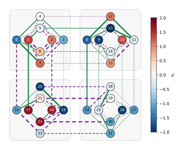
Random coefficients h and J on the Chimera graph

The color of a qubit shows $h_i$: red means $h_i>0$ and blue means $h_i<0$, and a darker color means a larger $|h_i|$. Since the term $h_is_i$ is negative when $s_i$ has the opposite sign to $h_i$, red qubits tend to take $-1$ and blue qubits tend to take $+1$.
Green solid lines are couplings with $J_{ij}<0$, which try to make the two spins equal (attract). Purple dashed lines are couplings with $J_{ij}>0$, which try to make the two spins opposite (repel). The width of a line shows the size of $|J_{ij}|$.

The second figure shows the solution of this problem:

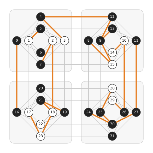
Solution of the Ising model on the Chimera graph

Black qubits have spin $+1$ and white qubits have spin $-1$. 23 of the 32 qubits take the direction preferred by $h_i$ (white for red, black for blue), but some, such as qubits 7 and 12, take the opposite direction because of their couplings. Thick orange lines are unsatisfied couplings, that is, couplings with $J_{ij}s_is_j>0$, which raise the energy when their terms are viewed alone. In general, no assignment satisfies all couplings at the same time. For example, if you go around a cycle and set each spin so that each coupling has the relation it prefers (equal or different), the direction may disagree when you come back to the start. The direction preferred by a field $h_i$ can also conflict with the direction preferred by the couplings. The optimal solution is the assignment that minimizes the total of these losses; in this example, 22 of the 80 couplings are unsatisfied.

Checking by exhaustive search

There are $2^{32}$ (about 4.3 billion) spin assignments for 32 qubits, so the Exhaustive Solver can check all of them. Change the two lines that create the solver and solve as follows:

solver = qbpp.ExhaustiveSolver(f)
sol = solver.search()

The output is the same as with EasySolver, which confirms that the EasySolver solution is the assignment with the minimum energy (the optimal solution). An ideal quantum annealer would also return this optimal solution. The exhaustive search took about 2 seconds on one GPU (A100) and about 30 seconds on 8 CPU cores alone.

Larger Chimera graphs

Setting ROWS and COLS to 16 gives 2048 qubits and 6016 couplings, the same as the 2000Q. Exhaustive search is impossible at this size, but EasySolver solves it as is. However, a time limit of 1 second may not reach the optimal solution, and a longer time limit may give a solution with lower energy.

Advantage2

The qubits of Advantage2 are coupled in the form of a Zephyr graph, which has more couplings than the Chimera graph (each qubit has at most 6 couplings in the Chimera graph and at most 20 in the Zephyr graph). The ranges of $h_i$ and $J_{ij}$ also differ from those of the 2000Q.

The part of this program that builds and solves the expression uses only nodes and edges returned by chimera() and the coefficients h and J. Therefore, if you use the nodes and edges of a Zephyr graph instead of chimera() and change the ranges of the random numbers to those of Advantage2, the same program simulates Advantage2. D-Wave’s Ocean SDK has functions that generate the lists of nodes and edges of Chimera and Zephyr graphs. Since a real machine may have qubits and couplings that cannot be used, you can obtain the lists of its qubits and couplings and the ranges of $h_i$ and $J_{ij}$ with the Ocean SDK and use them, so that PyQBPP solves a problem of the same form as that machine. In that case the qubit numbers have gaps, so create the variable array s with size “largest number + 1” (variables that do not appear in the expression do not affect the solution).