Traveling Salesman Problem
The Traveling Salesman Problem (TSP) asks for the shortest tour that visits every node exactly once and returns to the start. We assume that the nodes are placed on a plane and that the tour length is measured using the Euclidean distance.
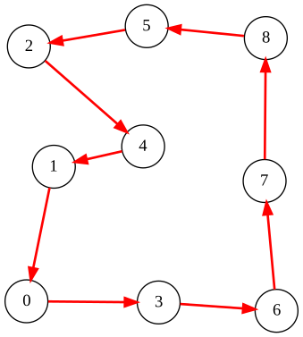
In the figure below, an example of nine nodes and an optimal tour is shown:
QUBO formulation of the TSP
A tour can be represented by a permutation of the nodes. Accordingly, we use a permutation matrix to encode a TSP solution.
Let $X=(x_{i,j})$ ($0\leq i,j\leq n-1$) be a matrix of $n\times n$ binary values. The matrix $X$ is a permutation matrix each row and each column contains exactly one entry equal to 1, as illustrated below.
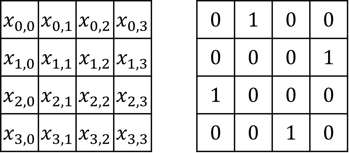
We interpret $x_{k,i}$ as “the $k$-th position in the tour is node $i$”. Therefore, every row and every column of $X$ must be one-hot, i.e., the following constraints must hold:
\[\begin{aligned} {\rm row}:& \sum_{j=0}^{n-1}x_{i,j}=1 & (0\leq i\leq n-1)\\ {\rm column}:& \sum_{i=0}^{n-1}x_{i,j}=1 & (0\leq j\leq n-1) \end{aligned}\]Let $d_{i,j}$ denote the distance between nodes $i$ and $j$. Then the tour length for a permutation matrix $X$ can be written as:
\[\begin{aligned} {\rm objective}: &\sum_{k=0}^{n-1}\sum_{i=0}^{n-1}\sum_{j=0}^{n-1} d_{i,j}x_{k,i}x_{(k+1)\bmod n,j} \end{aligned}\]This expression adds $d_{i,j}$ exactly when node $i$ is visited at position $k$ and node $j$ is visited next (at position $(k+1)\bmod n$), so it equals the total length of the tour.
PyQBPP program for TSP
Using the permutation-matrix formulation above, we can write a PyQBPP program for the TSP as follows:
import math
import pyqbpp as qbpp

nodes = [(10, 12),  (33, 125),  (12, 226),
         (121, 11), (108, 142), (111, 243),
         (220, 4),  (210, 113), (211, 233)]

def dist(i, j):
    dx = nodes[i][0] - nodes[j][0]
    dy = nodes[i][1] - nodes[j][1]
    return round(math.sqrt(dx * dx + dy * dy))

n = len(nodes)
x = qbpp.var("x", shape=(n, n))

constraint = qbpp.sum(qbpp.vector_sum(x, axis=1) == 1) + \
             qbpp.sum(qbpp.vector_sum(x, axis=0) == 1)

objective = 0
for i in range(n):
    next_i = (i + 1) % n
    for j in range(n):
        for k in range(n):
            if k != j:
                objective += dist(j, k) * x[i][j] * x[next_i][k]

f = objective + constraint * 1000
f.simplify_as_binary()

solver = qbpp.EasySolver(f)
sol = solver.search(time_limit=1.0)

# Convert the permutation matrix into a tour (list of node indices)
tour = []
for i in range(n):
    for j in range(n):
        if sol(x[i][j]) == 1:
            tour.append(j)
            break
print(f"Tour: {tour}")
In this program, the coordinates of nodes 0 through 8 are stored in the list nodes, and the helper function dist(i, j) computes the rounded Euclidean distance between two nodes. We create a 2D array x of binary variables and construct the one-hot constraints together with the tour-length objective. These terms are combined into a single QUBO expression f by adding the constraints with a penalty weight (here, 1000) to prioritize feasibility.
We then solve f using EasySolver with a 1.0-second time limit. The resulting assignment sol(x) forms a permutation matrix. This matrix is converted into a list of integers (a permutation) called tour by scanning each row for the entry equal to 1, and then printed.
This program produces the following output:
Tour: [7, 8, 5, 2, 4, 1, 0, 3, 6]
Optimizing exact (double) distances
The dist function above rounds each Euclidean distance to the nearest integer with round(), because the default coefficient type is integer. To optimize the exact tour length without rounding, use the double frontend: import pyqbpp.d and drop the round():
import pyqbpp.d as qbpp        # instead of: import pyqbpp as qbpp

def dist(i, j):
    dx = nodes[i][0] - nodes[j][0]
    dy = nodes[i][1] - nodes[j][1]
    return math.sqrt(dx * dx + dy * dy)   # no round()
The rest of the program is unchanged. The solver finds the same optimal tour, and sol.energy now returns the exact tour length as a float (e.g. 960.443) instead of the sum of rounded distances.
A more concise objective using slicing, concat, and einsum
The triple for-loop that builds objective is a direct translation of the formula $\sum_{i,j,k} d_{j,k}\, x_{i,j}\, x_{(i+1) \bmod n, k}$, but it can also be written as a single call to qbpp.einsum once two auxiliary arrays are prepared:
- a distance matrix
dof shape $n \times n$ withd[j, k] = dist(j, k), - a cyclically-shifted variable matrix
x_nextdefined byx_next[i, k] = x[(i+1) % n, k], built with slicing andconcat.
The objective then becomes the single line qbpp.einsum("jk,ij,ik->", d, x, x_next), replacing the entire triple loop:
# Distance matrix as a 2-D coefficient array
d = qbpp.array([dist(j, k) for j in range(n) for k in range(n)],
               shape=(n, n))

# Cyclic shift of x along axis 0:
#   x_next[i, k] = x[(i+1) % n, k]
x_next = qbpp.concat([x[1:], x[:1]], axis=0)

# Σ_{i,j,k} d[j,k] * x[i,j] * x_next[i,k]
objective = qbpp.einsum("jk,ij,ik->", d, x, x_next)
qbpp.array(..., shape=(n, n)) builds the $n \times n$ distance matrix from a flat list. x[1:] and x[:1] slice the rows of x, and qbpp.concat([...], axis=0) joins them so that x_next is x cyclically shifted by one row. The subscript "jk,ij,ik->" then contracts j and k between d and x_next and j between d and x, summing over i, j, k to yield the scalar objective.
The diagonal-skipping if k != j from the loop version is no longer needed: dist(j, j) is always 0, so those terms vanish automatically.
The resulting QUBO expression has the same set of terms as the for-loop version, but the construction is much shorter. It is also much faster for larger $n$, since the entire contraction runs inside the C++ backend with multithreading — avoiding the per-iteration Python ctypes overhead of the for-loop version.
Fixing the first node
Without loss of generality, we can assume that node 0 is the starting node of the tour. Because the TSP tour is invariant under cyclic shifts, fixing the start position does not change the optimal tour length.
By fixing the start node, we can reduce the number of binary variables in the QUBO expression. Specifically, we enforce that node 0 is assigned to position 0 in the permutation matrix. To do this, we fix the following binary variables:
\[\begin{aligned} x_{0,0} &= 1\\ x_{i,0} &= 0& (i\geq 1)\\ x_{0,j} &= 0& (j\geq 1) \end{aligned}\]These assignments ensure that node 0 appears only at position 0, and that no other node is assigned to position 0. As a result, the effective problem size is reduced, which generally makes the QUBO easier to solve for local-search–based solvers.
PyQBPP program for fixing the first node
In PyQBPP, fixed variable assignments can be applied using the qbpp.replace() function with a Python dict mapping variables to values:
ml = {x[0][0]: 1}
ml.update({x[i][0]: 0 for i in range(1, n)})
ml.update({x[0][i]: 0 for i in range(1, n)})

g = qbpp.replace(f, ml)
g.simplify_as_binary()

solver = qbpp.EasySolver(g)
sol = solver.search(time_limit=1.0)

full_sol = qbpp.Sol(f).set(sol, ml)

# Convert the permutation matrix into a tour (list of node indices)
tour = []
for i in range(n):
    for j in range(n):
        if full_sol(x[i][j]) == 1:
            tour.append(j)
            break
print(f"Tour: {tour}")
First, we create a Python dict ml, which stores fixed assignments of variables. Each key is a binary variable and each value is its fixed value (0 or 1).
Next, we call qbpp.replace(f, ml), which returns a new expression obtained by substituting the fixed values specified in ml into the original QUBO expression f. The resulting expression is stored in g and simplified.
We then create a solver for g and obtain a solution sol. Since sol corresponds to the reduced problem, we create a qbpp.Sol object for f and set both the solver output sol and the fixed assignments ml via set(sol, ml). The resulting full_sol stores the complete assignment for all variables in x.
Finally, the permutation matrix represented by full_sol(x) is converted into a permutation by scanning each row and printed.
This program produces the following tour starting from node 0:
Tour: [0, 3, 6, 7, 8, 5, 2, 4, 1]
Visualization using matplotlib
The following code visualizes the TSP solution, drawing each node as a labeled point and each tour edge as a directed red arrow:
import matplotlib.pyplot as plt

plt.figure(figsize=(6, 6))
for i, (nx_, ny) in enumerate(nodes):
    plt.plot(nx_, ny, "ko", markersize=8)
    plt.annotate(str(i), (nx_, ny), textcoords="offset points", xytext=(5, 5))

for i in range(n):
    fr = tour[i]
    to = tour[(i + 1) % n]
    plt.annotate("", xy=(nodes[to][0], nodes[to][1]),
                 xytext=(nodes[fr][0], nodes[fr][1]),
                 arrowprops=dict(arrowstyle="->", color="#e74c3c", lw=2))
plt.title("TSP Tour")
plt.savefig("tsp.png", dpi=150, bbox_inches="tight")
plt.show()
The tour is shown as directed red arrows connecting the nodes in visiting order.