Video: Nonogram (Python)
A companion to the video “QUBO++ Case Study: Nonogram (Python)”. For each chapter it gives the main points, the programs shown in the video with their output, and links to the pages that explain more. Click “▶ Play the video from …” to play from that scene. Programs that the video shows in parts are given here in full, ready to run.
What the video covers:
- The rules of the nonogram and a 15 × 15 puzzle whose answer is the QUBO++ logo
- Placing each block by its shift from the left-aligned position, with the shift as domain wall variables
- The order of the blocks as degree-2 penalty terms, and covering a cell as the difference of two strip values, so that the color of a cell is a linear expression
- Declaring with
qbpp.cons()that the row color equals the column color, solving it, and solving it as an expanded QUBO
The written explanation is on the page Nonogram. Back to the list of Videos (Case Studies)
Rules
The numbers to the left of the grid and above it list the lengths of the blocks of black cells of that row (column), from left to right (top to bottom). Between two blocks there is at least one white cell; the clue does not say how many white cells lie between the blocks or at the ends. This puzzle has 15 rows and 15 columns, and every row and column has black cells. It has only one answer.
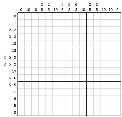
How far each block moves
As an example, we use the fifth row of the puzzle (clue 3 1 1 3, 15 cells, four blocks).
- With all blocks pushed to the left, blocks 0 to 3 start at $e = 0, 4, 6, 8$, and $d = 4$ cells, the margin, are left on the right.
- How far a block moves right from the left-aligned position is its shift $t$. In the answer, $t = (0, 1, 3, 4)$.
- A shift is between 0 and $d$, and blocks cannot pass each other, so a later block moves at least as far as an earlier one.
j   0  1  2  3  4  5  6  7  8  9 10 11 12 13 14
    #  #  #  .  #  .  #  .  #  #  #  .  .  .  .    t = (0, 0, 0, 0)  left-aligned
    #  #  #  .  .  #  .  .  .  #  .  .  #  #  #    t = (0, 1, 3, 4)  the answer
    .  .  .  .  #  #  #  .  #  .  #  .  #  #  #    t = (4, 4, 4, 4)  right-aligned
Domain walls
We restrict $d$ binary variables to patterns where every 1 comes before every 0 ($1\cdots 1\,0\cdots 0$), and regard the boundary as a wall. The number of 1s before the wall represents an integer from 0 to $d$ (with $d = 4$, the five patterns 0000 to 1111 represent 0 to 4; 1110 is 3).
- Flipping one variable moves the wall, changing the integer by one.
- Unlike counting 1s alone, each integer has exactly one pattern, so variable $p$ alone tells whether the integer is larger than $p$.
Shifts as domain walls
The shift of block $k$ is represented by four variables y[k, p] ($p = 0, \ldots, 3$); y[k, p] is 1 when the shift is larger than $p$. The answer’s shifts 0, 1, 3, 4 in a table with blocks as rows and $p$ as columns:
| $p=0$ | $p=1$ | $p=2$ | $p=3$ | |
|---|---|---|---|---|
| Block 0 ($t=0$) | 0 | 0 | 0 | 0 |
| Block 1 ($t=1$) | 1 | 0 | 0 | 0 |
| Block 2 ($t=3$) | 1 | 1 | 1 | 0 |
| Block 3 ($t=4$) | 1 | 1 | 1 | 1 |
- Each row is a domain wall (no 1 right after a 0). Where it breaks,
~y[k, p] * y[k, p + 1]is 1. - Each column, read from the top, is a domain wall in the opposite direction (no 0 below a 1). Where it breaks,
y[k, p] * ~y[k + 1, p]is 1. - Each product is 1 only where a shape breaks, so it can be used as a penalty term: the order of the blocks needs only degree-2 terms and no auxiliary variables.
When a block covers a cell
One block and one cell
We move block 3 (length $r = 3$, start $e = 8$) to the right and watch the cell at position 11.
| Shift $t$ | 0 | 1 | 2 | 3 | 4 |
|---|---|---|---|---|---|
| Block 3 at | 8–10 | 9–11 | 10–12 | 11–13 | 12–14 |
| Covers 11 | no | yes | yes | yes | no |
In general a block starts at $e+t$ and covers $r$ cells, so it covers position $j$ when $j-e-r < t \leq j-e$. Here that is $0 < t \leq 3$: shifts 1, 2 and 3.
Seen on the strip
Let $Y(q)$ be 1 if the shift is larger than $q$, and 0 otherwise.
- As $q$ goes up, $Y(q)$ stays 1 and turns 0 when $q$ reaches the shift: the strip of $Y$ values is a domain wall with its wall at the shift.
- For $0 \leq q \leq d-1$, $Y(q)$ is the variable
y[k, q]itself; for $q < 0$ it is 1 and for $q \geq d$ it is 0 (constants).
With markers $a = j-e-r$ and $b = j-e$ on the strip, the block covers the cell exactly when the wall is between $a$ and $b$.
| Wall | $Y(a)$ | $Y(b)$ | $Y(a)-Y(b)$ |
|---|---|---|---|
| Between $a$ and $b$ | 1 | 0 | 1 |
| Left of $a$ | 0 | 0 | 0 |
| Right of $b$ | 1 | 1 | 0 |
| (never) | 0 | 1 |
A 1 never follows a 0 on the strip, so the last row cannot happen. So the block covers the cell ⇔ $Y(a)-Y(b)=1$.
Checking with the example
With the answer’s shifts $(0, 1, 3, 4)$:
- Position 5: block 1 (length 1, start 4) has $a=0$, $b=1$. Its strip is 1000, so $Y(0)-Y(1)=1-0=1$. Block 1 covers it: black.
- Position 3: block 0 has $a=0$, $b=3$ and strip 0000, difference 0. For blocks 1 to 3, $a$ and $b$ are both negative, two constant 1s, difference 0. No block covers it: white.
Adding the differences of all the blocks gives the color of the cell seen from the row; blocks do not overlap, so the sum is 0 or 1. Each $Y$ is a variable or a constant, so the color is a linear expression of the variables (at position 5: y[0, 2] + y[1, 0] - y[1, 1]). With an integer variable for the shift, “larger than $q$” has no such formula.
See “Colors Seen from a Row” on the page Nonogram for more.
Matching rows and columns
Columns are handled the same way: the shift down from the top-aligned position, as domain wall variables z. The color seen from the column is linear in z. In every cell we require “row color − column color = 0” (225 equalities for the 225 cells). There are no auxiliary variables: just the 437 variables of y (198) and z (239). There is no objective, so the energy is 0 when every condition holds.
The program
The clues and three functions
- The clues are lists of lists:
ROWS[i]is the clue of row $i$ andCOLS[j]that of column $j$. line_varmakes the domain wall variables of one row (column): a 2-D array of blocks × margin, the table above.movedreturns the strip value $Y(q)$ (1 for negative $q$, 0 from $d$ on, the variable otherwise).blackgoes through the blocks, advancing the start positione, collectsmovedat $a$ minusmovedat $b$ for each block in a list, and adds them withqbpp.sum(): the color of the cell seen from the row.
The order conditions and solving
- In
line_cons, the first loop adds the row-shape penalty terms and the second loop the column-shape ones. yis the list of the row variable arrays andzthe list for the columns (the number of blocks and the margin differ from row to row).fgets the order conditions, andqbpp.cons()adds, for every cell, the constraint that the two colors differ by 0.- The terms contain negations, so
simplify_as_binary()tidies up, andEasySolversolves it withtarget_energy=0.
import pyqbpp as qbpp

# Clues: ROWS[i][k] is the length of the k-th block of row i,
# and COLS[j][k] is the length of the k-th block of column j.
ROWS = [[7], [11], [4, 4], [2, 2], [3, 1, 1, 3], [2, 3, 3, 2], [2, 1, 1, 2], [2, 2],
        [3, 3], [2, 2], [4, 4], [10], [7, 2], [4], [3]]
COLS = [[5], [9], [4, 4], [2, 2], [3, 1, 3], [2, 3, 2], [2, 1, 2], [2, 2],
        [2, 1, 2], [2, 3, 2], [3, 1, 3], [2, 2, 1], [4, 3, 3], [9, 3], [5, 2]]
H, W = len(ROWS), len(COLS)


# Domain walls w[k, p] of a row (column) of length n: they represent the shift of block k.
def line_var(name, clue, n):
    d = n - sum(clue) - len(clue) + 1  # margin
    return qbpp.var(name, shape=(len(clue), d))


# Expression that is 1 if the shift of block k is greater than q.
def moved(w, k, q):
    if q < 0:
        return 1
    if q >= w.shape[1]:
        return 0
    return w[k, q]


# Expression that is 1 if position j is black.
def black(w, clue, j):
    b = []
    e = 0  # left-aligned (top-aligned) start position of block k
    for k in range(len(clue)):
        b.append(moved(w, k, j - e - clue[k]) - moved(w, k, j - e))
        e += clue[k] + 1
    return qbpp.sum(b)


# Constraints of one row (column).
def line_cons(w):
    m, d = w.shape
    g = 0
    for k in range(m):
        for p in range(d - 1):
            g += ~w[k, p] * w[k, p + 1]  # domain wall form (1 if a 1 follows a 0)
    for k in range(m - 1):
        for p in range(d):
            g += w[k, p] * ~w[k + 1, p]  # block order (1 if a 0 is below a 1)
    return g


y = [line_var(f"y{i}", ROWS[i], W) for i in range(H)]  # domain walls of row i
z = [line_var(f"z{j}", COLS[j], H) for j in range(W)]  # domain walls of column j

f = 0
for w in y + z:
    f += line_cons(w)
for i in range(H):
    for j in range(W):
        f += qbpp.cons(black(y[i], ROWS[i], j) - black(z[j], COLS[j], i) == 0)  # the colors of the row and the column match

f.simplify_as_binary()
sol = qbpp.EasySolver(f).search(target_energy=0)
for i in range(H):
    print("".join("#" if sol(black(y[i], ROWS[i], j)) else "." for j in range(W)))
Running it
Laying the # and . of the output over the grid shows the QUBO++ logo. There is only one answer, so every run prints the same:
....#######....
..###########..
.####.....####.
.##.........##.
###..#...#..###
##..###.###..##
##...#...#...##
##...........##
###.........###
.##.........##.
.####.....####.
..##########...
....#######.##.
...........####
............###
Solving it as a QUBO
qbpp.expand_cons() expands the constraints declared with qbpp.cons() into penalties. An equality becomes (row color − column color)², which has degree 2 because both colors are linear. The order conditions are degree-2 penalty terms from the start. The expanded expression is a QUBO without auxiliary variables, and its energy is 0 only when every condition holds. Add these lines at the end of the program above:
g = qbpp.expand_cons(f)
g.simplify_as_binary()
sol = qbpp.EasySolver(g).search(target_energy=0)
print(f"var_count = {sol.info['var_count']}, term_count = {sol.info['term_count']}")
Output:
var_count = 437, term_count = 2756
There are still 437 variables, and 2756 terms. In this form it can be passed to any solver that takes a QUBO.
See “Solving as a QUBO” on the page Nonogram for more.
Summary
- Each block’s position became its shift from the left-aligned position, and each shift became domain wall variables.
- The order of the blocks became degree-2 penalty terms.
- Covering a cell became the difference of two strip values, so the color of a cell is a linear expression of the variables.
- An equality between the row color and the column color ties rows and columns together, with no auxiliary variables; expanding it gives a QUBO directly.