Video: Simulating a Quantum Annealer (Python)
A companion to the video “QUBO++ Case Study: Simulating a Quantum Annealer (Python)”. For each chapter it gives the main points, the programs shown in the video with their output, and links to the pages that explain more. Click “▶ Play the video from …” to play from that scene. Programs that the video shows in part are given here in full, ready to run.
What the video covers:
- The energy of the Ising model that a quantum annealer solves, and the Chimera graph, the coupling layout of the 2000Q
- Turning an expression written with spin variables into an expression of binary variables (a QUBO) with
spin_to_binary() - Solving a randomly generated problem on 2 × 2 cells (32 qubits) with EasySolver
- Why not every coupling can be satisfied, and checking with an exhaustive search by ExhaustiveSolver that the answer is optimal
- Scaling up to 16 × 16 cells, the Zephyr graph of Advantage2, and the three topologies Chimera, Pegasus and Zephyr
Back to the list of Videos (Case Studies)
Quantum annealers
A quantum annealer is a device that, on a graph with a fixed coupling layout, searches for spin assignments with low Ising model energy. Writing the same Ising model in QUBO++ and solving it gives the answer the annealer is expected to return, without the real machine. Simulation in this video means getting the answer this way, not imitating the quantum dynamics. Use it to test a program before a real run, or to compare the machine’s answers with the optimum.
The Ising model
Qubit $i$ represents a spin $s_i \in \lbrace -1, +1 \rbrace$. The energy is the sum of the field terms and the coupling terms.
\[E(s) = \sum_{i} h_i s_i + \sum_{(i,j)} J_{ij}\, s_i s_j\]- A positive $h_i$ lowers the energy with a spin down ($-1$); a negative $h_i$, with a spin up ($+1$).
- A coupling with negative $J_{ij}$ tries to align the two spins; one with positive $J_{ij}$ tries to make them opposite.
- On the 2000Q, $h_i$ is from $-2$ to $2$, and $J_{ij}$ from $-1$ to $1$.
In a small example with three spins ($h = (0.5, 0.5, -1)$, $J_{01} = -1$, $J_{12} = 0.5$), all five terms are negative for $s = (-1, -1, +1)$, and the sum $-3.5$ is the smallest of the 8 assignments.
The Chimera graph
The qubits of the 2000Q are coupled in the form of a Chimera graph, a grid of cells of 8 qubits.
- The 8 qubits of a cell form two groups of 4: group 0 and group 1.
- In a cell, every qubit of group 0 couples to every qubit of group 1 (16 edges).
- Group 0 couples to group 0 at the same position in the cell below, and group 1 to group 1 at the same position in the cell to the right.
2 × 2 cells give 32 qubits and 80 couplings. The 2000Q had 16 × 16 cells (2048 qubits). Qubit $k$ of group $u$ in the cell at row $i$, column $j$ gets the number $((i \cdot C + j) \cdot 2 + u) \cdot 4 + k$ ($C$ is the number of cell columns); for example, qubit 2 of group 1 in the cell at row 1, column 0 is 22. This is the same numbering as in the Chimera graphs of the Ocean SDK.
See Simulating a Quantum Annealer for more.
Converting to QUBO
PyQBPP solvers solve expressions of binary variables, 0 or 1. Writing a spin $s_i$ with a binary variable $x_i$ as $s_i = 2x_i - 1$ ($+1$ if $x_i = 1$, $-1$ if $x_i = 0$) makes $E(s)$ an expression of binary variables. For the three-spin example it is the following, and its value agrees with the original $E(s)$ for all 8 assignments.
\[f(x) = 3x_0 + 2x_1 - 3x_2 - 4x_0x_1 + 2x_1x_2 - 0.5\]In PyQBPP, write $E(s)$ with spin variables and call spin_to_binary(). The substituted expression has the same value as the original $E(s)$, so the energy the solver returns is exactly the energy of the Ising model.
See QR: Operations for more.
The program
The function chimera()
The function chimera(rows, cols) builds the Chimera graph of rows by cols cells and returns nodes, the list of qubit numbers, and edges, the list of couplings. The inner function q computes the number of a qubit, and three kinds of couplings go into edges: inside a cell, vertical ones to the cell below, and horizontal ones to the cell to the right. With ROWS and COLS at 2, the graph has 32 qubits and 80 couplings.
import random
import pyqbpp.d as qbpp


def chimera(rows, cols):
    L = 4  # number of qubits in each group of a cell

    def q(i, j, u, k):
        return ((i * cols + j) * 2 + u) * L + k

    nodes = list(range(rows * cols * 2 * L))
    edges = []
    for i in range(rows):
        for j in range(cols):
            for k in range(L):
                for l in range(L):
                    edges.append((q(i, j, 0, k), q(i, j, 1, l)))
                if i + 1 < rows:
                    edges.append((q(i, j, 0, k), q(i + 1, j, 0, k)))
                if j + 1 < cols:
                    edges.append((q(i, j, 1, k), q(i, j + 1, 1, k)))
    return nodes, edges


ROWS, COLS = 2, 2  # numbers of cell rows and columns
nodes, edges = chimera(ROWS, COLS)
Build f from random h and J, and solve it with EasySolver
import pyqbpp.dmakes the coefficients of expressions real numbers (float).- The fields
hare uniform random numbers from $-2$ to $2$ and the couplingsJfrom $-1$ to $1$, held in dictionaries per qubit and per coupling. The random seed is 1, so the problem is the same every time. - With spin variables
s, $E(s)$ becomes the expressionf;spin_to_binary()turns it into an expression of binary variables, andsimplify_as_binary()simplifies it. - EasySolver solves it with a time limit of 1 second, and
2 * sol(s[v]) - 1turns the values back into spins. $E(s)$ is recomputed with these spins and printed next tosol.energy.
import random
import pyqbpp.d as qbpp


def chimera(rows, cols):
    L = 4  # number of qubits in each group of a cell

    def q(i, j, u, k):
        return ((i * cols + j) * 2 + u) * L + k

    nodes = list(range(rows * cols * 2 * L))
    edges = []
    for i in range(rows):
        for j in range(cols):
            for k in range(L):
                for l in range(L):
                    edges.append((q(i, j, 0, k), q(i, j, 1, l)))
                if i + 1 < rows:
                    edges.append((q(i, j, 0, k), q(i + 1, j, 0, k)))
                if j + 1 < cols:
                    edges.append((q(i, j, 1, k), q(i, j + 1, 1, k)))
    return nodes, edges


ROWS, COLS = 2, 2  # numbers of cell rows and columns
nodes, edges = chimera(ROWS, COLS)

random.seed(1)
h = {v: random.uniform(-2, 2) for v in nodes}
J = {e: random.uniform(-1, 1) for e in edges}

s = qbpp.var("s", shape=len(nodes))
f = 0
for v in nodes:
    f += h[v] * s[v]
for (a, b), w in J.items():
    f += w * s[a] * s[b]
f.spin_to_binary()
f.simplify_as_binary()

solver = qbpp.EasySolver(f)
sol = solver.search(time_limit=1)

spin = {v: 2 * sol(s[v]) - 1 for v in nodes}
E = 0
for v in nodes:
    E += h[v] * spin[v]
for (a, b), w in J.items():
    E += w * spin[a] * spin[b]
print(f"energy = {sol.energy:.4f}")
print(f"E(s)   = {E:.4f}")
for i in range(ROWS):
    for j in range(COLS):
        v = (i * COLS + j) * 8
        left = " ".join(f"{spin[v + k]:+d}" for k in range(4))
        right = " ".join(f"{spin[v + k]:+d}" for k in range(4, 8))
        print(f"cell ({i},{j}): {left} | {right}")
See Simulating a Quantum Annealer for more.
Results
The output
The output in the video (EasySolver may give different results on each run):
energy = -46.2007
E(s)   = -46.2007
cell (0,0): +1 -1 -1 -1 | +1 +1 +1 +1
cell (0,1): +1 +1 -1 +1 | +1 +1 -1 -1
cell (1,0): +1 -1 -1 +1 | +1 +1 -1 -1
cell (1,1): +1 +1 +1 +1 | -1 -1 +1 +1
energy and E(s) agree: the energy of the solver is exactly the energy of the Ising model. The other 4 lines are the spins of the 8 qubits of each cell, group 0 to the left of | and group 1 to the right.
The problem and its solution
The first figure is the problem, and the second is the solution.
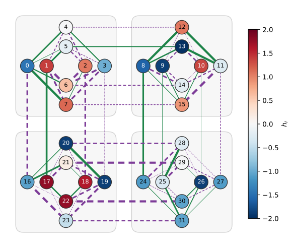
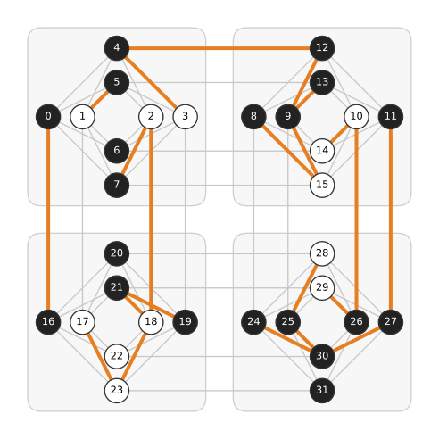
- The problem: a qubit’s color is $h_i$, red for positive, blue for negative, darker for a larger absolute value. Green solid lines are attracting couplings ($J_{ij} < 0$), purple dashed lines repelling ones ($J_{ij} > 0$); the thicker a line, the larger $\lvert J_{ij} \rvert$.
- The solution: black is spin $+1$ and white is $-1$. 23 of the 32 qubits take the direction their $h_i$ prefers (white for red, black for blue), but qubits 7 and 12 are red yet black: their couplings pull them the other way.
- Thick orange lines are unsatisfied couplings; their terms alone would raise the energy.
Why not every coupling can be satisfied
In the cycle 7 → 1 → 6 → 2 → 7 of the top-left cell, start with 7 as $+1$ and set each spin the way its coupling wants: 1 becomes $-1$, 6 becomes $+1$ and 2 becomes $-1$. The last coupling, 2 and 7, attracts, so it wants 7 to be $-1$ too; but 7 started as $+1$, so after one lap the directions disagree. In a cycle with an odd number of repelling couplings, one coupling cannot be satisfied. The optimum breaks only the cycle’s weakest coupling, 2 and 7. The field may also prefer a direction the couplings do not, and the optimum is the assignment with the smallest total loss. In this example, 22 of the 80 couplings are not satisfied.
Checking with exhaustive search
32 qubits have $2^{32}$ (about 4.3 billion) assignments, so ExhaustiveSolver can check all of them. We only change the two solving lines to qbpp.ExhaustiveSolver(f) and search().
import random
import pyqbpp.d as qbpp


def chimera(rows, cols):
    L = 4  # number of qubits in each group of a cell

    def q(i, j, u, k):
        return ((i * cols + j) * 2 + u) * L + k

    nodes = list(range(rows * cols * 2 * L))
    edges = []
    for i in range(rows):
        for j in range(cols):
            for k in range(L):
                for l in range(L):
                    edges.append((q(i, j, 0, k), q(i, j, 1, l)))
                if i + 1 < rows:
                    edges.append((q(i, j, 0, k), q(i + 1, j, 0, k)))
                if j + 1 < cols:
                    edges.append((q(i, j, 1, k), q(i, j + 1, 1, k)))
    return nodes, edges


ROWS, COLS = 2, 2  # numbers of cell rows and columns
nodes, edges = chimera(ROWS, COLS)

random.seed(1)
h = {v: random.uniform(-2, 2) for v in nodes}
J = {e: random.uniform(-1, 1) for e in edges}

s = qbpp.var("s", shape=len(nodes))
f = 0
for v in nodes:
    f += h[v] * s[v]
for (a, b), w in J.items():
    f += w * s[a] * s[b]
f.spin_to_binary()
f.simplify_as_binary()

solver = qbpp.ExhaustiveSolver(f)
sol = solver.search()

spin = {v: 2 * sol(s[v]) - 1 for v in nodes}
E = 0
for v in nodes:
    E += h[v] * spin[v]
for (a, b), w in J.items():
    E += w * spin[a] * spin[b]
print(f"energy = {sol.energy:.4f}")
print(f"E(s)   = {E:.4f}")
for i in range(ROWS):
    for j in range(COLS):
        v = (i * COLS + j) * 8
        left = " ".join(f"{spin[v + k]:+d}" for k in range(4))
        right = " ".join(f"{spin[v + k]:+d}" for k in range(4, 8))
        print(f"cell ({i},{j}): {left} | {right}")
Output:
energy = -46.2007
E(s)   = -46.2007
cell (0,0): +1 -1 -1 -1 | +1 +1 +1 +1
cell (0,1): +1 +1 -1 +1 | +1 +1 -1 -1
cell (1,0): +1 -1 -1 +1 | +1 +1 -1 -1
cell (1,1): +1 +1 +1 +1 | -1 -1 +1 +1
The output is exactly the same as with EasySolver, so the EasySolver solution is the assignment with the minimum energy: the optimum. An ideal quantum annealer would also return this optimum. In the video, the exhaustive search took about 2 seconds on one GPU (A100) and about 30 seconds on 8 CPU cores alone.
See Exhaustive Solver for more.
Larger Chimera graphs and Advantage2
With ROWS and COLS at 16, the graph has 2048 qubits and 6016 couplings, as on the 2000Q. Exhaustive search is impossible, but EasySolver solves it as is. A time limit of 1 second may not reach the optimum, though; a longer one may give a solution with lower energy.
import random
import pyqbpp.d as qbpp


def chimera(rows, cols):
    L = 4  # number of qubits in each group of a cell

    def q(i, j, u, k):
        return ((i * cols + j) * 2 + u) * L + k

    nodes = list(range(rows * cols * 2 * L))
    edges = []
    for i in range(rows):
        for j in range(cols):
            for k in range(L):
                for l in range(L):
                    edges.append((q(i, j, 0, k), q(i, j, 1, l)))
                if i + 1 < rows:
                    edges.append((q(i, j, 0, k), q(i + 1, j, 0, k)))
                if j + 1 < cols:
                    edges.append((q(i, j, 1, k), q(i, j + 1, 1, k)))
    return nodes, edges


ROWS, COLS = 16, 16  # numbers of cell rows and columns
nodes, edges = chimera(ROWS, COLS)

random.seed(1)
h = {v: random.uniform(-2, 2) for v in nodes}
J = {e: random.uniform(-1, 1) for e in edges}

s = qbpp.var("s", shape=len(nodes))
f = 0
for v in nodes:
    f += h[v] * s[v]
for (a, b), w in J.items():
    f += w * s[a] * s[b]
f.spin_to_binary()
f.simplify_as_binary()

solver = qbpp.EasySolver(f)
sol = solver.search(time_limit=1)

spin = {v: 2 * sol(s[v]) - 1 for v in nodes}
E = 0
for v in nodes:
    E += h[v] * spin[v]
for (a, b), w in J.items():
    E += w * spin[a] * spin[b]
print(f"energy = {sol.energy:.4f}")
print(f"E(s)   = {E:.4f}")
for i in range(ROWS):
    for j in range(COLS):
        v = (i * COLS + j) * 8
        left = " ".join(f"{spin[v + k]:+d}" for k in range(4))
        right = " ".join(f"{spin[v + k]:+d}" for k in range(4, 8))
        print(f"cell ({i},{j}): {left} | {right}")
The output in the video (EasySolver gives different results on each run):
energy = -2883.4410
E(s)   = -2883.4410
cell (0,0): +1 -1 -1 +1 | -1 +1 -1 -1
...
Advantage2 uses the Zephyr graph, with more couplings than the Chimera graph, and its ranges of $h_i$ and $J_{ij}$ differ from those of the 2000Q.
- The part that builds and solves the expression uses only
nodes,edgesand the coefficientshandJ. - Using the
nodesandedgesof a Zephyr graph instead ofchimera(), with the ranges of the random numbers changed too, the same program simulates Advantage2. - The real machine’s qubits and couplings, and the ranges of the coefficients, come from the Ocean SDK. When some qubits cannot be used and the numbers have gaps, make
sof size “largest number + 1”; the unused numbers do not affect the solution.
See Simulating a Quantum Annealer for more.
Three topologies
For the topologies of three generations of D-Wave quantum annealers, we count the couplings of one qubit (the layouts are the ones drawn by the Ocean SDK).
| Quantum annealer | Topology | Most couplings of a qubit |
|---|---|---|
| 2000Q | Chimera graph | 6 |
| Advantage | Pegasus graph | 15 |
| Advantage2 | Zephyr graph | 20 |
With each generation, the couplings become denser. For any of the graphs, passing nodes and edges lets the same program solve it.
Summary
- We wrote the energy of the Ising model directly with spin variables.
spin_to_binary()turned it into an expression of binary variables.pyqbpp.dhandled the real coefficients.- EasySolver solved it, and ExhaustiveSolver confirmed that the answer is optimal.
- The expression is built from
nodes,edgesand the coefficients only, so it works for other graphs too. - We also compared the three topologies Chimera, Pegasus and Zephyr.